Assignment 4: Linear Programming, Game Theory, and R Code Solutions
VerifiedAdded on 2022/10/06
|9
|2184
|13
Homework Assignment
AI Summary
This assignment solution addresses several problems related to linear programming and game theory. The first question involves optimizing production costs using linear programming with two variables, solved graphically using Desmos. The second question formulates and solves a linear programming problem with multiple variables, using R code to maximize profit given constraints on demand and material proportions. The third question explores a two-player zero-sum game, formulating the payoff matrix, identifying the absence of a saddle point, and developing R code to find the optimal strategies for both players. Finally, the fourth question analyzes a game theory scenario to determine the Nash equilibrium for two companies, also discussing how changes in cost affect the optimal strategy. The assignment demonstrates an understanding of linear programming, game theory, and their practical applications, including the use of R for computation.

Assignment 4
ASSIGNMENT 4
by[Name]
Course
Professor’s Name
Institution
Location of Institution
Date
ASSIGNMENT 4
by[Name]
Course
Professor’s Name
Institution
Location of Institution
Date
Paraphrase This Document
Need a fresh take? Get an instant paraphrase of this document with our AI Paraphraser
Assignment 4
Assignment 4
Question 1
(a) The problem has a number of restrictions on the amount of lime, orange and mango
used in each product A and B. The other restriction is on the total cost of each product
and the minimum liters of beverage the customers require. These restrictions can be
expressible in quantitative terms (Adler, Papadimitriou and Rubinstein 2014). Next,
the prices of product A and product B (inputs) for the manufacture of the beverage are
both constant. There exist an objective of minimizing cost and the relationship
between objective function and constraints are linear (Dyer et al. 2017). Finally,
negative units of product A or B cannot be used to produce a beverage therefore, the
assumptions of linear program are all satisfied by the problem.
(b) Let the food factory use x = liters of product A and y liters of product B in producing
(x + y) liters of the beverage for the customer giving a total cost.
C = 5x + 7y.
The restriction on the production inform of an equation are as follows:
Orange Mango Lime
3 x+ 2 y ≥ 225, 2 x+3 y ≥ 250, 3x +8 y ≤ 600
Non-negativity - x ≥ 0 and y≥ 0.
Therefore, the linear program is
Min C = 5x + 7y.
Subject to:
3 x+ 2 y ≥ 225, 2 x+3 y ≥ 250, 3x +8 y ≤ 600, x + y ≥ 80, x ≥ 0, and y≥ 0
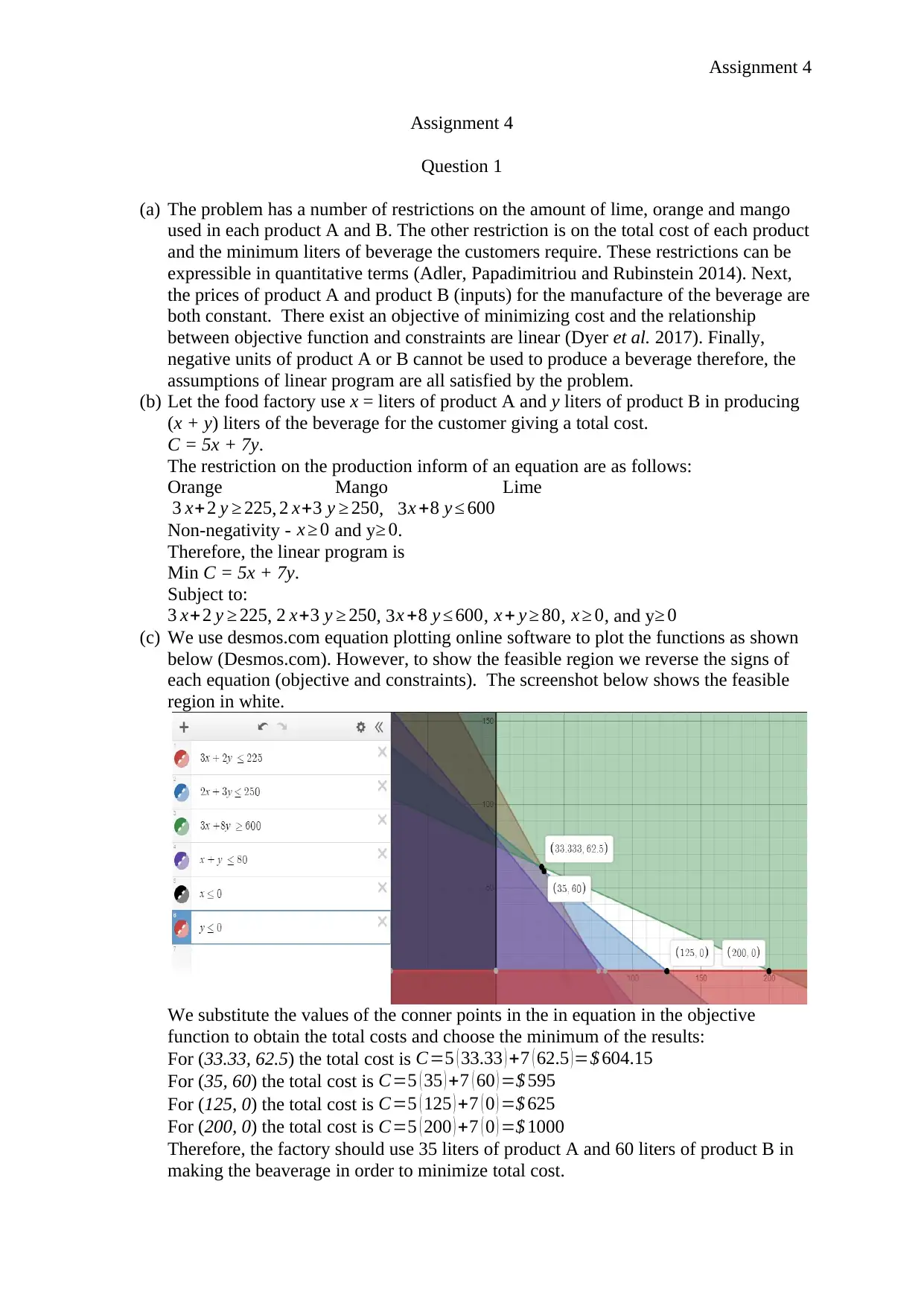
(c) We use desmos.com equation plotting online software to plot the functions as shown
below (Desmos.com). However, to show the feasible region we reverse the signs of
each equation (objective and constraints). The screenshot below shows the feasible
region in white.
We substitute the values of the conner points in the in equation in the objective
function to obtain the total costs and choose the minimum of the results:
For (33.33, 62.5) the total cost is C=5 ( 33.33 ) +7 ( 62.5 )=$ 604.15
For (35, 60) the total cost is C=5 ( 35 ) +7 ( 60 ) =$ 595
For (125, 0) the total cost is C=5 ( 125 ) +7 ( 0 ) =$ 625
For (200, 0) the total cost is C=5 ( 200 ) +7 ( 0 ) =$ 1000
Therefore, the factory should use 35 liters of product A and 60 liters of product B in
making the beaverage in order to minimize total cost.
Assignment 4
Question 1
(a) The problem has a number of restrictions on the amount of lime, orange and mango
used in each product A and B. The other restriction is on the total cost of each product
and the minimum liters of beverage the customers require. These restrictions can be
expressible in quantitative terms (Adler, Papadimitriou and Rubinstein 2014). Next,
the prices of product A and product B (inputs) for the manufacture of the beverage are
both constant. There exist an objective of minimizing cost and the relationship
between objective function and constraints are linear (Dyer et al. 2017). Finally,
negative units of product A or B cannot be used to produce a beverage therefore, the
assumptions of linear program are all satisfied by the problem.
(b) Let the food factory use x = liters of product A and y liters of product B in producing
(x + y) liters of the beverage for the customer giving a total cost.
C = 5x + 7y.
The restriction on the production inform of an equation are as follows:
Orange Mango Lime
3 x+ 2 y ≥ 225, 2 x+3 y ≥ 250, 3x +8 y ≤ 600
Non-negativity - x ≥ 0 and y≥ 0.
Therefore, the linear program is
Min C = 5x + 7y.
Subject to:
3 x+ 2 y ≥ 225, 2 x+3 y ≥ 250, 3x +8 y ≤ 600, x + y ≥ 80, x ≥ 0, and y≥ 0
(c) We use desmos.com equation plotting online software to plot the functions as shown
below (Desmos.com). However, to show the feasible region we reverse the signs of
each equation (objective and constraints). The screenshot below shows the feasible
region in white.
We substitute the values of the conner points in the in equation in the objective
function to obtain the total costs and choose the minimum of the results:
For (33.33, 62.5) the total cost is C=5 ( 33.33 ) +7 ( 62.5 )=$ 604.15
For (35, 60) the total cost is C=5 ( 35 ) +7 ( 60 ) =$ 595
For (125, 0) the total cost is C=5 ( 125 ) +7 ( 0 ) =$ 625
For (200, 0) the total cost is C=5 ( 200 ) +7 ( 0 ) =$ 1000
Therefore, the factory should use 35 liters of product A and 60 liters of product B in
making the beaverage in order to minimize total cost.
Assignment 4
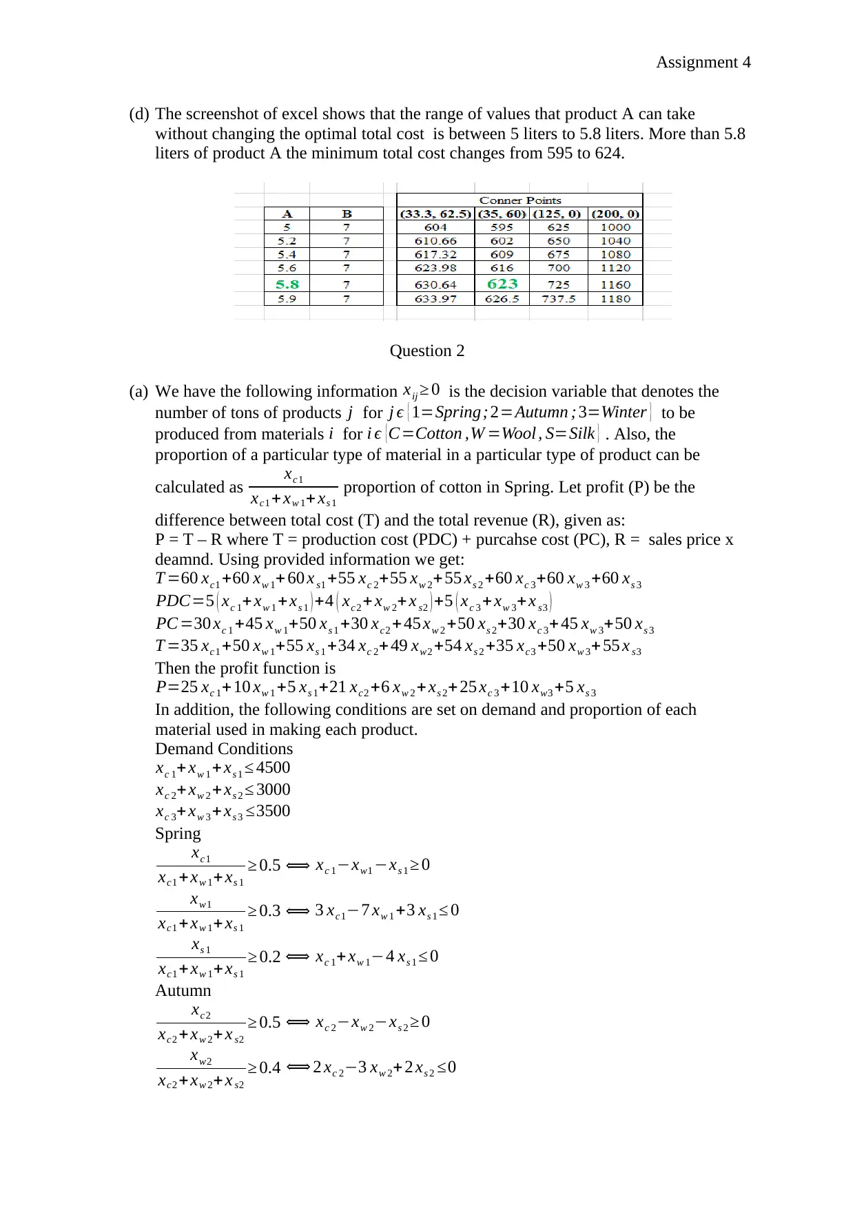
(d) The screenshot of excel shows that the range of values that product A can take
without changing the optimal total cost is between 5 liters to 5.8 liters. More than 5.8
liters of product A the minimum total cost changes from 595 to 624.
Question 2
(a) We have the following information xij ≥ 0 is the decision variable that denotes the
number of tons of products j for j ϵ { 1=Spring; 2=Autumn ;3=Winter } to be
produced from materials i for i ϵ {C=Cotton ,W =Wool , S=Silk } . Also, the
proportion of a particular type of material in a particular type of product can be
calculated as xc1
xc1 + xw 1+ xs 1
proportion of cotton in Spring. Let profit (P) be the
difference between total cost (T) and the total revenue (R), given as:
P = T – R where T = production cost (PDC) + purcahse cost (PC), R = sales price x
deamnd. Using provided information we get:
T =60 xc1 +60 xw 1+ 60 x s1 +55 xc 2+55 xw 2+55 xs 2 +60 xc 3+60 xw 3 +60 xs 3
PDC=5 ( xc 1+ xw 1 + xs 1 ) +4 ( xc2 + xw 2+ x s2 ) +5 ( xc 3 + xw 3+x s3 )
PC =30 xc 1 +45 xw 1+50 xs 1 +30 xc2 + 45 xw 2 +50 xs 2+30 xc 3+ 45 xw 3+50 xs 3
T =35 xc1 +50 xw 1+55 xs 1 +34 xc 2+ 49 xw2 +54 xs 2 +35 xc3 +50 xw 3+ 55 x s3
Then the profit function is
P=25 xc 1+ 10 xw 1 +5 xs 1+21 xc2 +6 xw 2 + xs 2+ 25 xc 3 +10 xw3 +5 xs 3
In addition, the following conditions are set on demand and proportion of each
material used in making each product.
Demand Conditions
xc 1+xw 1 + xs 1 ≤ 4500
xc 2+ xw 2 +xs 2 ≤ 3000
xc 3+xw 3 + xs 3 ≤3500
Spring
xc1
xc1 +xw 1+ xs 1
≥ 0.5 ⟺ xc 1−xw1 −xs 1 ≥ 0
xw1
xc1 + xw 1+ xs 1
≥ 0.3 ⟺ 3 xc1−7 xw 1 +3 xs 1 ≤ 0
xs 1
xc1 + xw 1+xs 1
≥ 0.2 ⟺ xc 1+ xw 1−4 xs 1 ≤ 0
Autumn
xc2
xc2 + xw 2+ x s2
≥ 0.5 ⟺ xc 2−xw 2−xs 2 ≥ 0
xw2
xc2 +xw 2+ x s2
≥ 0.4 ⟺ 2 xc 2−3 xw 2+ 2 xs 2 ≤0
⊘ This is a preview!⊘
Do you want full access?
Subscribe today to unlock all pages.
Trusted by 1+ million students worldwide
Assignment 4
xs 2
xc2 + xw 2+x s2
≥ 0.1 ⟺ xc2 +xw 2−9 xs 2 ≤0
Winter
xc3
xc3 + xw 3+ xs 3
≥ 0.4 ⟺ 3 xc3−2 xw 3−2 xs 3 ≥ 0
xw3
xc3 + xw 3+ xs 3
≥ 0.5 ⟺ xc 3−xw 3+x s3 ≤ 0
xs 3
xc3 + xw 3+ xs 3
≥ 0.1 ⟺ xc 3+xw 3−9 x s3 ≤ 0
Non-negativity constraints
xc 1 ≥ 0 , xc 2 ≥ 0 , xc3 ≥ 0 , xs 1 ≥ 0 , xs 2 ≥0 , xs 3 ≥0 , xw 1 ≥ 0 , xw2 ≥ 0 , xw 3 ≥0
Therefore,
Max P=25 xc 1+10 xw 1 +5 xs 1+21 xc2 +6 xw 2 + xs 2+ 25 xc 3 +10 xw3 +5 xs 3 Subject to:
xc 1+xw 1 + xs 1 ≤ 4500
xc 2+ xw 2 +xs 2 ≤ 3000
xc 3+xw 3 + xs 3 ≤3500
xc 1−xw1 −xs 1 ≥ 0
3 xc1−7 xw 1 +3 xs 1 ≤ 0
xc 1+ xw 1−4 xs 1 ≤ 0
xc 2−xw 2−xs 2 ≥ 0
2 xc2−3 xw 2 +2 xs 2 ≤ 0
xc 2+ xw 2−9 xs 2 ≤ 0
3 xc3 −2 xw 3−2 xs 3 ≥ 0
xc 3−xw 3+ x s3 ≤ 0
xc 3+xw 3−9 x s3 ≤ 0
xij ≥ 0
(b) The R-code is as follows:
## load the package
library(lpSolve)
## Objective function
ObjecFunction <- c(25, 50, 55, 34, 49, 54, 35, 50, 55)
## Constraint matrix
ConstraintMatrix <- matrix(c(rep(1,3), rep(0,6),
rep(0,3), rep(1,3), rep(0,3),
rep(0,6), rep(1,3),
1,-1,-1, rep(0,6),3,-7,3, rep(0,6),
1,1,-4, rep(0,6),rep(0,3),
1,-1,-1, rep(0,6),2,-3,2,rep(0,6),
1,1,-9,rep(0,9),3,-2,-2, rep(0,6),
1,-1,1,rep(0,6),1,1,-9,diag(9)),
nrow = 21, ncol = 9, byrow = TRUE)
## Constraint dircetions
ConstraintDirection <- c(rep("<=",3), ">=",rep("<=",2),
">=",rep("<=",2),">=",rep("<=",2),rep(">=",9))
## Create constraint right hand side values
ConstraintRhs <- c(4500,3000,3500, rep(0, 18))
## Solve the linear program
Paraphrase This Document
Need a fresh take? Get an instant paraphrase of this document with our AI Paraphraser
Assignment 4
Optimize <- lp("max", ObjecFunction, ConstraintMatrix,
ConstraintDirection, ConstraintRhs, compute.sens=T)
## solutions
Optimize$objval
Optimize$solution
The maximum profit is $455,000 while the optimal value of the decision variables
are xc 1=¿2250, xw 1=¿1350, xs 1=¿900, xc 2=¿1500, xw 2=¿1200, xs 2=¿300 ,
xc 3=¿400, xw 3=¿1750, and xs 3=¿350.
Question 3
(a) The game requires that the amount lost by the first is gained by the second player.
There are only two players, Hellen and David and at each stage of either David wins
or Hellen wins. The loser gets a negative score while the winner gets a postive score
(De Paula 2013; Morris 2012). The sum of the scores at each play is equal to zero.
Therefore, the game satisfy the conditions needed for it to be a two-player zero-sum
game.
(b) In formulation of the payoff matrix we suppose the following David (row player) and
Hellen Column player. Next, let i strategy choosen by David and j be strategy choosen
by Hellen. From hint i=1 , 2 ,… , 7 and j=1 ,2 , … , 6. Where, the payoff matrix A is
shown below.
David (i)
Hellen( j)
(−5
0
0
−5 0 0
−5 −5 0
0 −5 −10
0 −5 −5
−5 −5 0
−5 0 0
0
0
−5
0 −5 −10
−5 −5 0
−5 0 0
−5 0 0
−5 −5 0
0 −5 −5
)(c) “A saddle point (pure Nashs equilibrium) of a payoff matrix A is a pair ( i¿ , j¿ ) such
that:”
max
i
ai j¿=ai¿ j¿=min
j
ai¿ j
Where aij is the payoff (the amount the winner receives) (Karlin and Peres 2016,
p.38). Identification of saddle point in the payoff matrix A require us to find row
minimax and column maximin. A saddle point exist if the two values are equal. The
row minimax is -5 while the column maximin is zero. There does not exist a saddle
point.
(d) Let David pick strategy i with probability pi and Hellen pick strategy j with
probability q j.
Throughout, p= ( p1 , p2 ,… , p7 )' and q= ( q1 ,q2 ,.. , q6 )' . Where;
p7=1− ( p1 +p2+ p3+ p4 + p5 + p6 ) and q6=1− ( q1 +q2+ q3 +q4 +q5 )
Finally let’s define the payoff as v.
The linear program for David is
Objective is to max v
Subject to:
−v e1 +Ap ≥ 0 (i)
0 ≤ pi ≤ 1 (ii)
Assignment 4
∑
i=1
7
pi =1 (iii)
The linear program for Hellen is
Objective is to min v
Subject to:
−v e2 +A' q ≥0
qi ≥ 0
∑
i=1
6
qi=1
Where: e1= ( 1 ,1 , 1 ,1 , 1 ,1 )' and e2= ( 1 , 1, 1 ,1 , 1 ,1 , 1 )'
(e) Equation (i) can be expandend to form a 6 x 8 matrix as follows:
−v−5 p1−5 p2−5 p6−5 (1− ( q1+ q2 +q3+ q4 +q5 ) ) ≥ 0
−v+5 p3 +5 p4 +5 p5−5≥ 0
−v−5 p2−5 p3−5 p5−5 p6 ≥ 0
−v−5 p3−10 p4 −5 p5 ≥ 0
−v−5 p3−10 p4 −5 p5 ≥ 0
−v−5 p2−5 p3−5 p5−5 p6 ≥ 0
−v−5 p1−5 p2−5 p6−5 (1− ( q1+ q2 +q3+ q4 +q5 ) ) ≥ 0
−v+5 p3 +5 p4 +5 p5−5≥ 0
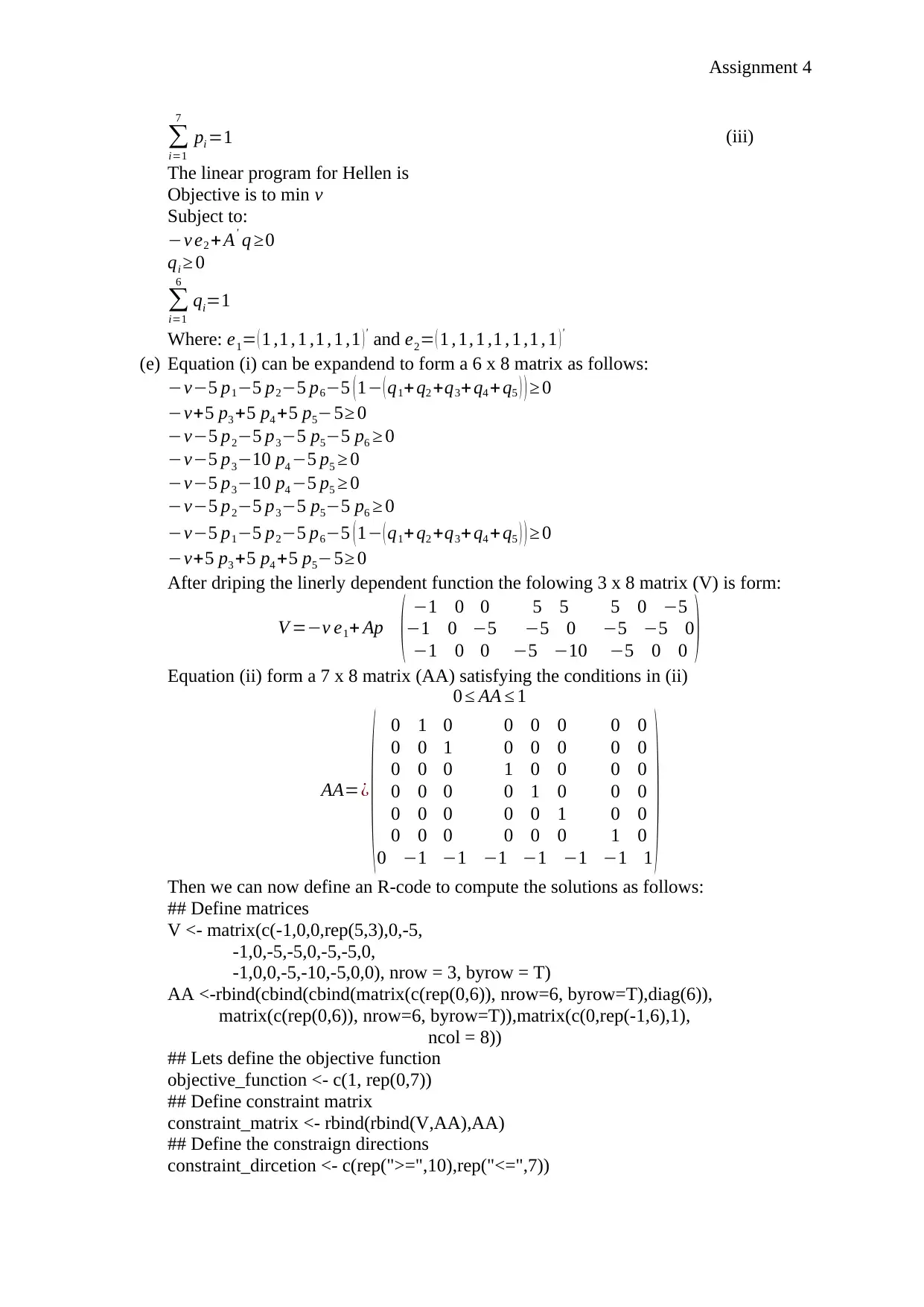
After driping the linerly dependent function the folowing 3 x 8 matrix (V) is form:
V =−v e1+ Ap ( −1 0 0 5 5 5 0 −5
−1 0 −5 −5 0 −5 −5 0
−1 0 0 −5 −10 −5 0 0 )
Equation (ii) form a 7 x 8 matrix (AA) satisfying the conditions in (ii)
0 ≤ AA ≤ 1
AA=¿
( 0 1 0
0 0 1
0 0 0
0 0 0
0 0 0
1 0 0
0 0
0 0
0 0
0 0 0
0 0 0
0 0 0
0 1 0
0 0 1
0 0 0
0 0
0 0
1 0
0 −1 −1 −1 −1 −1 −1 1
)Then we can now define an R-code to compute the solutions as follows:
## Define matrices
V <- matrix(c(-1,0,0,rep(5,3),0,-5,
-1,0,-5,-5,0,-5,-5,0,
-1,0,0,-5,-10,-5,0,0), nrow = 3, byrow = T)
AA <-rbind(cbind(cbind(matrix(c(rep(0,6)), nrow=6, byrow=T),diag(6)),
matrix(c(rep(0,6)), nrow=6, byrow=T)),matrix(c(0,rep(-1,6),1),
ncol = 8))
## Lets define the objective function
objective_function <- c(1, rep(0,7))
## Define constraint matrix
constraint_matrix <- rbind(rbind(V,AA),AA)
## Define the constraign directions
constraint_dircetion <- c(rep(">=",10),rep("<=",7))
∑
i=1
7
pi =1 (iii)
The linear program for Hellen is
Objective is to min v
Subject to:
−v e2 +A' q ≥0
qi ≥ 0
∑
i=1
6
qi=1
Where: e1= ( 1 ,1 , 1 ,1 , 1 ,1 )' and e2= ( 1 , 1, 1 ,1 , 1 ,1 , 1 )'
(e) Equation (i) can be expandend to form a 6 x 8 matrix as follows:
−v−5 p1−5 p2−5 p6−5 (1− ( q1+ q2 +q3+ q4 +q5 ) ) ≥ 0
−v+5 p3 +5 p4 +5 p5−5≥ 0
−v−5 p2−5 p3−5 p5−5 p6 ≥ 0
−v−5 p3−10 p4 −5 p5 ≥ 0
−v−5 p3−10 p4 −5 p5 ≥ 0
−v−5 p2−5 p3−5 p5−5 p6 ≥ 0
−v−5 p1−5 p2−5 p6−5 (1− ( q1+ q2 +q3+ q4 +q5 ) ) ≥ 0
−v+5 p3 +5 p4 +5 p5−5≥ 0
After driping the linerly dependent function the folowing 3 x 8 matrix (V) is form:
V =−v e1+ Ap ( −1 0 0 5 5 5 0 −5
−1 0 −5 −5 0 −5 −5 0
−1 0 0 −5 −10 −5 0 0 )
Equation (ii) form a 7 x 8 matrix (AA) satisfying the conditions in (ii)
0 ≤ AA ≤ 1
AA=¿
( 0 1 0
0 0 1
0 0 0
0 0 0
0 0 0
1 0 0
0 0
0 0
0 0
0 0 0
0 0 0
0 0 0
0 1 0
0 0 1
0 0 0
0 0
0 0
1 0
0 −1 −1 −1 −1 −1 −1 1
)Then we can now define an R-code to compute the solutions as follows:
## Define matrices
V <- matrix(c(-1,0,0,rep(5,3),0,-5,
-1,0,-5,-5,0,-5,-5,0,
-1,0,0,-5,-10,-5,0,0), nrow = 3, byrow = T)
AA <-rbind(cbind(cbind(matrix(c(rep(0,6)), nrow=6, byrow=T),diag(6)),
matrix(c(rep(0,6)), nrow=6, byrow=T)),matrix(c(0,rep(-1,6),1),
ncol = 8))
## Lets define the objective function
objective_function <- c(1, rep(0,7))
## Define constraint matrix
constraint_matrix <- rbind(rbind(V,AA),AA)
## Define the constraign directions
constraint_dircetion <- c(rep(">=",10),rep("<=",7))
⊘ This is a preview!⊘
Do you want full access?
Subscribe today to unlock all pages.
Trusted by 1+ million students worldwide
Assignment 4
## Define constraint right hand side
constraint_rhs <- c(rep(0,9),1,rep(0,6),1)
## Load the parckage for analysisng LP
library(lpSolve)
solution <- lp("max",objective_function, constraint_matrix, constraint_dircetion,
constraint_rhs, compute.sens = T)
solution$objval
solution$solution
(f) The game is biased since there is not strategy that David can choose for him to win
aginst Hellen, the best he can get is a draw of losing nothing (Morris 2012).
Question 4
(a) Let Profiti be the profit of company i for i∈ { 1=company 1 , 2=company 2 }
We have been given:
Q1=200−P1− ( P1−P )∧Q2=200−P2− ( P2 −P ) where P= P1 + P2
2 . The two equations
can simplify to
Q1=200−1.5 P1+0.5 P2 and Q2=200+ 0.5 P1 −1.5 P2
The profit from sale of each cellphone are:
P1=70 P2=70
Profitcompany 1= ( 200−1.5 ( 70 ) +0.5 ( 70 ) ) x 55=7,150
Profitcompany 2= ( 200+0.5 ( 70 ) −1.5 ( 70 ) ) x 55=7,150
P1=70 P2=80
Profitcompany 1= ( 200−1.5 ( 70 )+ 0.5 ( 80 ) ) x 55=7,425
Profitcompany 2= ( 200+ 0.5 ( 70 ) −1.5 ( 80 ) ) x 65=7,475
P1=70 P2=90
Profitcompany 1= ( 200−1.5 ( 70 ) + 0.5 ( 90 ) ) x 55=7,700
Profitcompany 2= ( 200+0.5 ( 70 ) −1.5 ( 90 ) ) x 75=7,500
P1=80 P2=70
Profitcompany 1= ( 200−1.5 ( 80 ) +0.5 ( 70 ) ) x 65=7,475
Profitcompany 2= ( 200+ 0.5 ( 80 ) −1.5 ( 70 ) ) x 55=7,425
P1=80 P2=80
Profitcompany 1= ( 200−1.5 ( 80 ) +0.5 ( 80 ) ) x 65=7,800
Profitcompany 2= ( 200+ 0.5 ( 80 )−1.5 ( 80 ) ) x 65=7,800
P1=80 P2=90
Profitcompany 1= ( 200−1.5 ( 80 ) +0.5 ( 90 ) ) x 65=8,125
Profitcompany 2= ( 200+ 0.5 ( 80 ) −1.5 ( 90 ) ) x 75=7,875
P1=90 P2=70
Profitcompany 1= ( 200−1.5 ( 90 ) +0.5 ( 70 ) ) x 75=7,500
Profitcompany 2= ( 200+0.5 ( 90 ) −1.5 ( 70 ) ) x 55=7,700
P1=90 P2=80
Profitcompany 1= ( 200−1.5 ( 90 ) +0.5 ( 80 ) ) x 75=7.875
Paraphrase This Document
Need a fresh take? Get an instant paraphrase of this document with our AI Paraphraser
Assignment 4
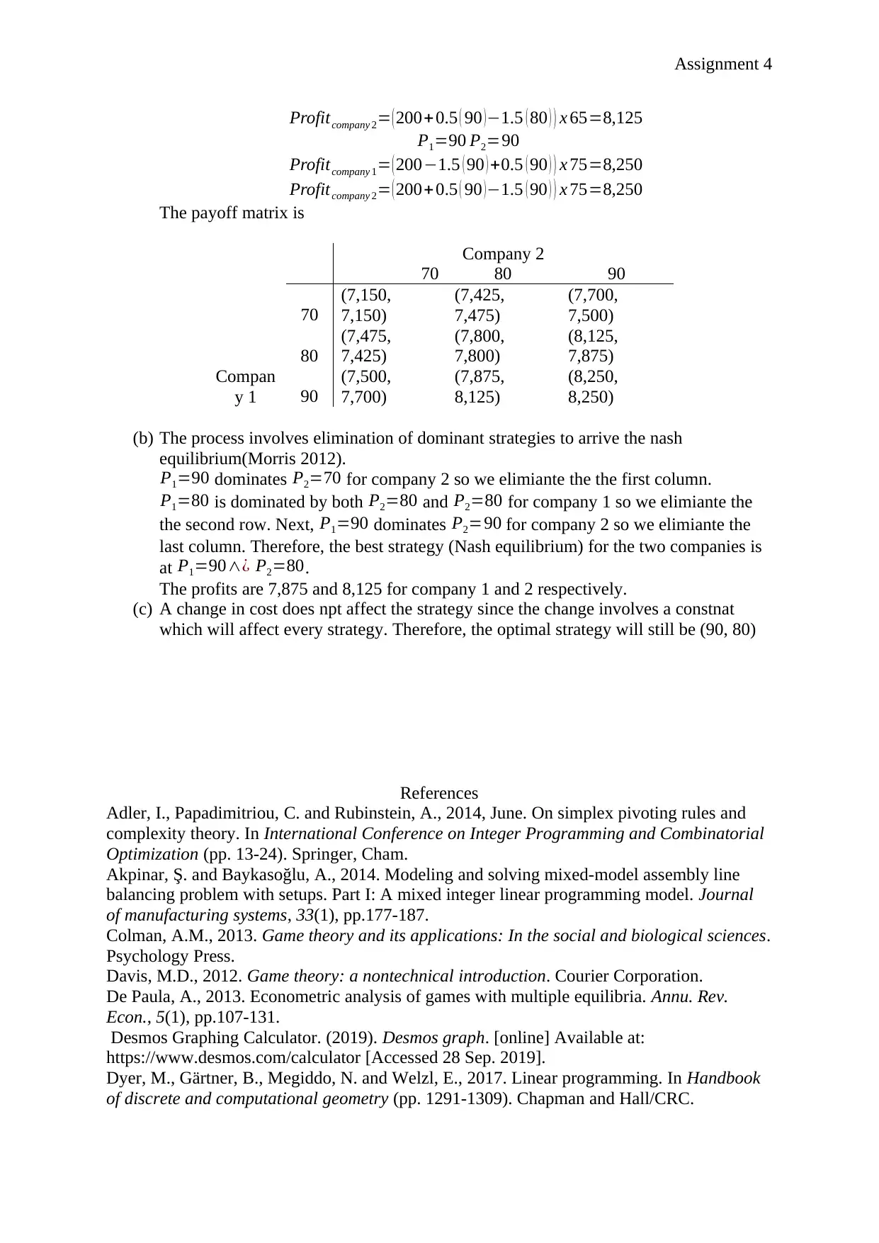
Profitcompany 2= ( 200+ 0.5 ( 90 )−1.5 ( 80 ) ) x 65=8,125
P1=90 P2=90
Profitcompany 1= ( 200−1.5 ( 90 ) +0.5 ( 90 ) ) x 75=8,250
Profitcompany 2= ( 200+ 0.5 ( 90 ) −1.5 ( 90 ) ) x 75=8,250
The payoff matrix is
Compan
y 1
Company 2
70 80 90
70
(7,150,
7,150)
(7,425,
7,475)
(7,700,
7,500)
80
(7,475,
7,425)
(7,800,
7,800)
(8,125,
7,875)
90
(7,500,
7,700)
(7,875,
8,125)
(8,250,
8,250)
(b) The process involves elimination of dominant strategies to arrive the nash
equilibrium(Morris 2012).
P1=90 dominates P2=70 for company 2 so we elimiante the the first column.
P1=80 is dominated by both P2=80 and P2=80 for company 1 so we elimiante the
the second row. Next, P1=90 dominates P2=90 for company 2 so we elimiante the
last column. Therefore, the best strategy (Nash equilibrium) for the two companies is
at P1=90∧¿ P2=80.
The profits are 7,875 and 8,125 for company 1 and 2 respectively.
(c) A change in cost does npt affect the strategy since the change involves a constnat
which will affect every strategy. Therefore, the optimal strategy will still be (90, 80)
References
Adler, I., Papadimitriou, C. and Rubinstein, A., 2014, June. On simplex pivoting rules and
complexity theory. In International Conference on Integer Programming and Combinatorial
Optimization (pp. 13-24). Springer, Cham.
Akpinar, Ş. and Baykasoğlu, A., 2014. Modeling and solving mixed-model assembly line
balancing problem with setups. Part I: A mixed integer linear programming model. Journal
of manufacturing systems, 33(1), pp.177-187.
Colman, A.M., 2013. Game theory and its applications: In the social and biological sciences.
Psychology Press.
Davis, M.D., 2012. Game theory: a nontechnical introduction. Courier Corporation.
De Paula, A., 2013. Econometric analysis of games with multiple equilibria. Annu. Rev.
Econ., 5(1), pp.107-131.
Desmos Graphing Calculator. (2019). Desmos graph. [online] Available at:
https://www.desmos.com/calculator [Accessed 28 Sep. 2019].
Dyer, M., Gärtner, B., Megiddo, N. and Welzl, E., 2017. Linear programming. In Handbook
of discrete and computational geometry (pp. 1291-1309). Chapman and Hall/CRC.

Assignment 4
Ge, R., Huang, F., Jin, C. and Yuan, Y., 2015, June. Escaping from saddle points—online
stochastic gradient for tensor decomposition. In Conference on Learning Theory (pp. 797-
842).
Higle, J.L. and Sen, S., 2013. Stochastic decomposition: a statistical method for large scale
stochastic linear programming (Vol. 8). Springer Science & Business Media.
Mansini, R., Ogryczak, W. and Speranza, M.G., 2014. Twenty years of linear programming
based portfolio optimization. European Journal of Operational Research, 234(2), pp.518-
535.
Morris, P., 2012. Introduction to game theory. Springer Science & Business Media.
Recht, B., Re, C., Tropp, J. and Bittorf, V., 2012. Factoring nonnegative matrices with linear
programs. In Advances in Neural Information Processing Systems (pp. 1214-1222).
⊘ This is a preview!⊘
Do you want full access?
Subscribe today to unlock all pages.
Trusted by 1+ million students worldwide
1 out of 9
Related Documents


![Course Name: Real World Analytics Assignment Solution - [Date]](/_next/image/?url=https%3A%2F%2Fdesklib.com%2Fmedia%2Fimages%2Fjs%2F7cd677b2bca5453d86bfbb121190a9b2.jpg&w=256&q=75)
Your All-in-One AI-Powered Toolkit for Academic Success.
+13062052269
info@desklib.com
Available 24*7 on WhatsApp / Email
![[object Object]](/_next/static/media/star-bottom.7253800d.svg)
Unlock your academic potential
Copyright © 2020–2026 A2Z Services. All Rights Reserved. Developed and managed by ZUCOL.