Comprehensive Solutions for Linear Programming Problems Analysis

This document presents detailed solutions to three linear programming (LP) problems. Problem A involves maximizing an objective function subject to resource constraints, solved using the simplex method to find the optimal solution for x1, x2, and x3. Problem B addresses a similar maximization problem, incorporating artificial variables in a two-phase approach to handle constraints, ultimately determining the optimal values for x1, x2, and x3. Problem C delves into sensitivity analysis, determining shadow prices and ranges of optimality for the objective function coefficients and right-hand-side values. The analysis includes examining the impact of changes in objective function coefficients for both basic and non-basic variables to maintain the optimal solution.

Problems of Linear Programming
1

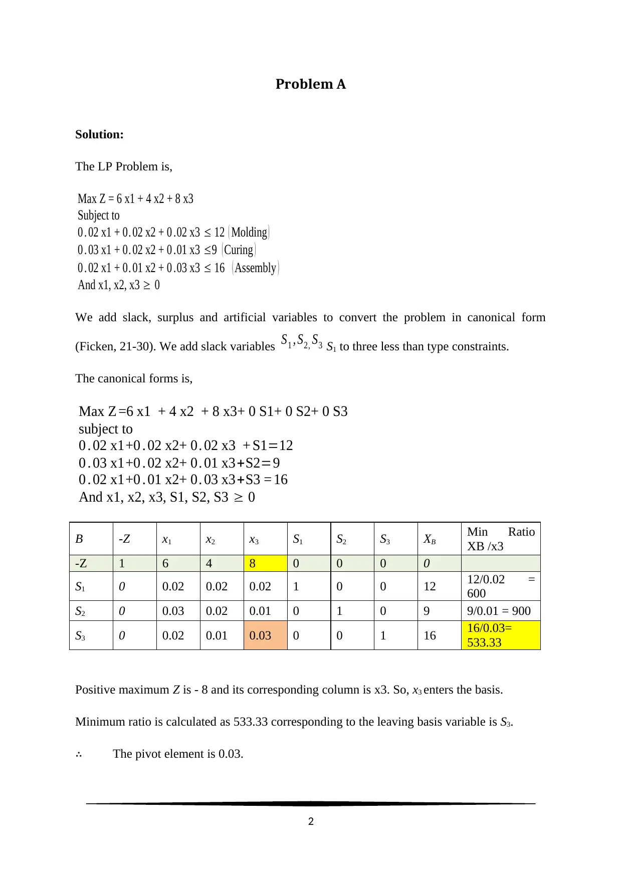
Problem A
Solution:
The LP Problem is,
Max Z = 6 x1 + 4 x2 + 8 x3
Subject to
0 . 02 x1 + 0. 02 x2 + 0 .02 x3 ≤ 12 ( Molding )
0 . 03 x1 + 0. 02 x2 + 0 .01 x3 ≤9 ( Curing )
0 . 02 x1 + 0. 01 x2 + 0 .03 x3 ≤ 16 ( Assembly )
And x1, x2, x3 ≥ 0
We add slack, surplus and artificial variables to convert the problem in canonical form
(Ficken, 21-30). We add slack variables S1 , S2, S3 S1 to three less than type constraints.
The canonical forms is,
Max Z =6 x1 + 4 x2 + 8 x3+ 0 S1+ 0 S2+ 0 S3
subject to
0 . 02 x1+0 . 02 x2+ 0. 02 x3 + S1=12
0 . 03 x1+0 . 02 x2+ 0. 01 x3+S2=9
0 . 02 x1+0 . 01 x2+ 0. 03 x3+S3 = 16
And x1, x2, x3, S1, S2, S3 ≥ 0
B -Z x1 x2 x3 S1 S2 S3 XB
Min Ratio
XB /x3
-Z 1 6 4 8 0 0 0 0
S1 0 0.02 0.02 0.02 1 0 0 12 12/0.02 =
600
S2 0 0.03 0.02 0.01 0 1 0 9 9/0.01 = 900
S3 0 0.02 0.01 0.03 0 0 1 16 16/0.03=
533.33
Positive maximum Z is - 8 and its corresponding column is x3. So, x3 enters the basis.
Minimum ratio is calculated as 533.33 corresponding to the leaving basis variable is S3.
∴ The pivot element is 0.03.
2

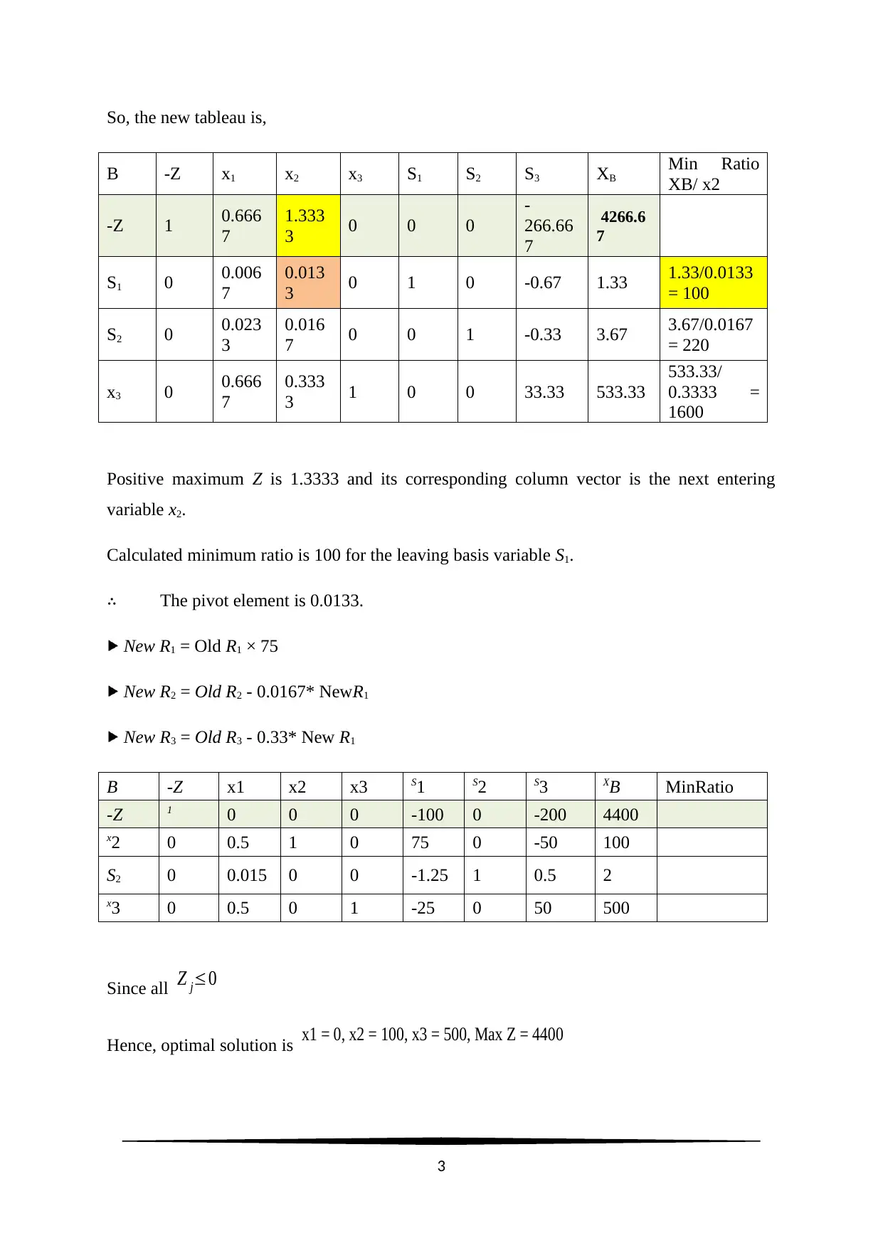
So, the new tableau is,
B -Z x1 x2 x3 S1 S2 S3 XB
Min Ratio
XB/ x2
-Z 1 0.666
7
1.333
3 0 0 0
-
266.66
7
4266.6
7
S1 0 0.006
7
0.013
3 0 1 0 -0.67 1.33 1.33/0.0133
= 100
S2 0 0.023
3
0.016
7 0 0 1 -0.33 3.67 3.67/0.0167
= 220
x3 0 0.666
7
0.333
3 1 0 0 33.33 533.33
533.33/
0.3333 =
1600
Positive maximum Z is 1.3333 and its corresponding column vector is the next entering
variable x2.
Calculated minimum ratio is 100 for the leaving basis variable S1.
∴ The pivot element is 0.0133.
New R1 = Old R1 × 75
New R2 = Old R2 - 0.0167* NewR1
New R3 = Old R3 - 0.33* New R1
B -Z x1 x2 x3 S1 S2 S3 XB MinRatio
-Z 1 0 0 0 -100 0 -200 4400
x2 0 0.5 1 0 75 0 -50 100
S2 0 0.015 0 0 -1.25 1 0.5 2
x3 0 0.5 0 1 -25 0 50 500
Since all Z j≤0
Hence, optimal solution is x1 = 0, x2 = 100, x3 = 500, Max Z = 4400
3

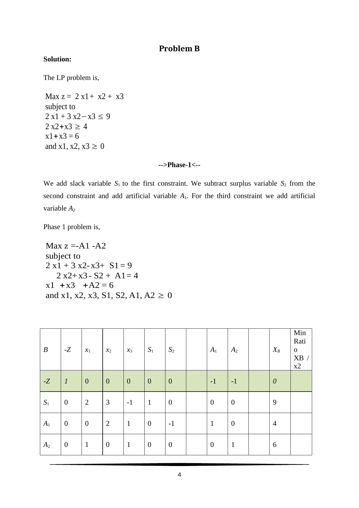
Problem B
Solution:
The LP problem is,
Max z = 2 x1 + x2 + x3
subject to
2 x1 + 3 x2−x3 ≤ 9
2 x2+x3 ≥ 4
x1+ x3 = 6
and x1, x2, x3 ≥ 0
-->Phase-1<--
We add slack variable S1 to the first constraint. We subtract surplus variable S2 from the
second constraint and add artificial variable A1. For the third constraint we add artificial
variable A2
Phase 1 problem is,
Max z =-A1 -A2
subject to
2 x1 + 3 x2- x3+ S1 = 9
2 x2+ x3 - S2 + A1= 4
x1 + x3 +A2 = 6
and x1, x2, x3, S1, S2, A1, A2 ≥ 0
B -Z x1 x2 x3 S1 S2 A1 A2 XB
Min
Rati
o
XB /
x2
-Z 1 0 0 0 0 0 -1 -1 0
S1 0 2 3 -1 1 0 0 0 9
A1 0 0 2 1 0 -1 1 0 4
A2 0 1 0 1 0 0 0 1 6
4

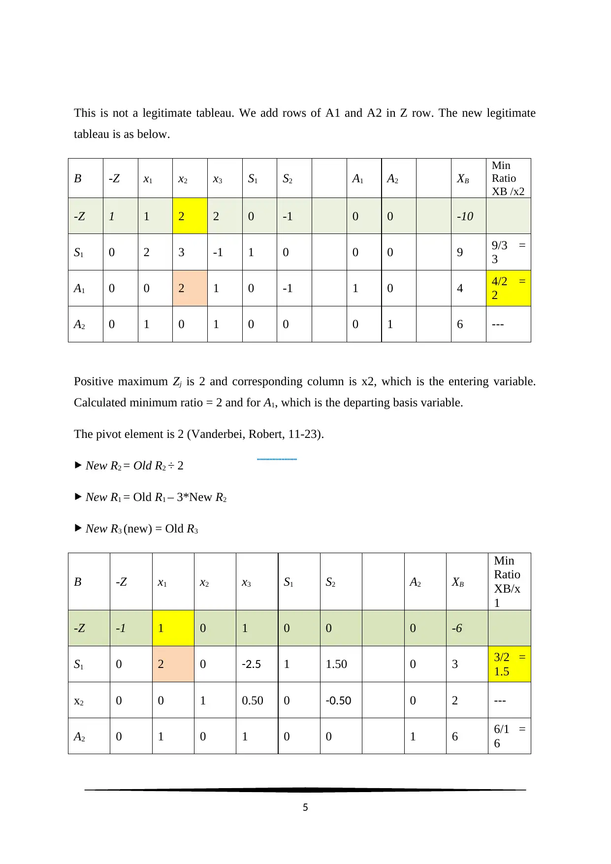
This is not a legitimate tableau. We add rows of A1 and A2 in Z row. The new legitimate
tableau is as below.
B -Z x1 x2 x3 S1 S2 A1 A2 XB
Min
Ratio
XB /x2
-Z 1 1 2 2 0 -1 0 0 -10
S1 0 2 3 -1 1 0 0 0 9 9/3 =
3
A1 0 0 2 1 0 -1 1 0 4 4/2 =
2
A2 0 1 0 1 0 0 0 1 6 ---
Positive maximum Zj is 2 and corresponding column is x2, which is the entering variable.
Calculated minimum ratio = 2 and for A1, which is the departing basis variable.
The pivot element is 2 (Vanderbei, Robert, 11-23).
New R2 = Old R2 ÷ 2
New R1 = Old R1 – 3*New R2
New R3 (new) = Old R3
B -Z x1 x2 x3 S1 S2 A2 XB
Min
Ratio
XB/x
1
-Z -1 1 0 1 0 0 0 -6
S1 0 2 0 -2.5 1 1.50 0 3 3/2 =
1.5
x2 0 0 1 0.50 0 -0.50 0 2 ---
A2 0 1 0 1 0 0 1 6 6/1 =
6
5

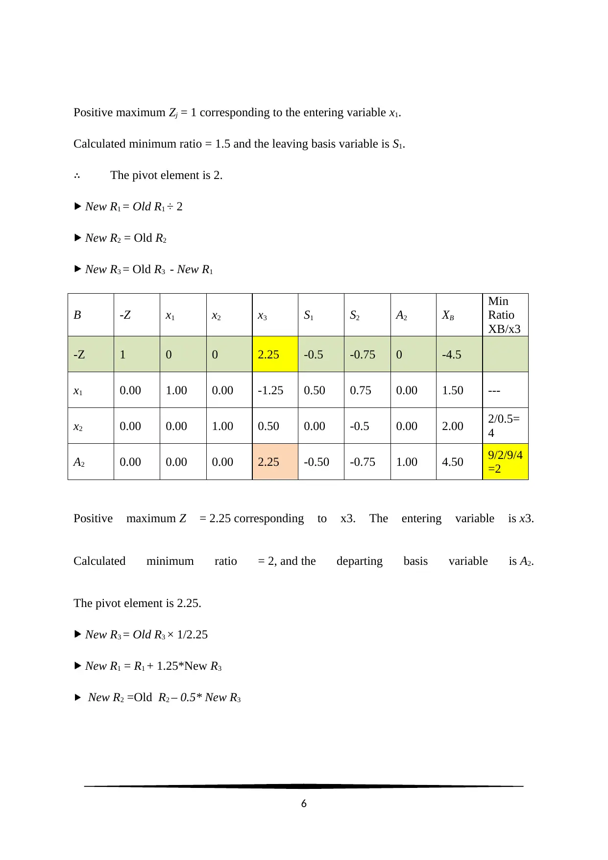
Positive maximum Zj = 1 corresponding to the entering variable x1.
Calculated minimum ratio = 1.5 and the leaving basis variable is S1.
∴ The pivot element is 2.
New R1 = Old R1 ÷ 2
New R2 = Old R2
New R3 = Old R3 - New R1
B -Z x1 x2 x3 S1 S2 A2 XB
Min
Ratio
XB/x3
-Z 1 0 0 2.25 -0.5 -0.75 0 -4.5
x1 0.00 1.00 0.00 -1.25 0.50 0.75 0.00 1.50 ---
x2 0.00 0.00 1.00 0.50 0.00 -0.5 0.00 2.00 2/0.5=
4
A2 0.00 0.00 0.00 2.25 -0.50 -0.75 1.00 4.50 9/2/9/4
=2
Positive maximum Z = 2.25 corresponding to x3. The entering variable is x3.
Calculated minimum ratio = 2, and the departing basis variable is A2.
The pivot element is 2.25.
New R3 = Old R3 × 1/2.25
New R1 = R1 + 1.25*New R3
New R2 =Old R2 – 0.5* New R3
6

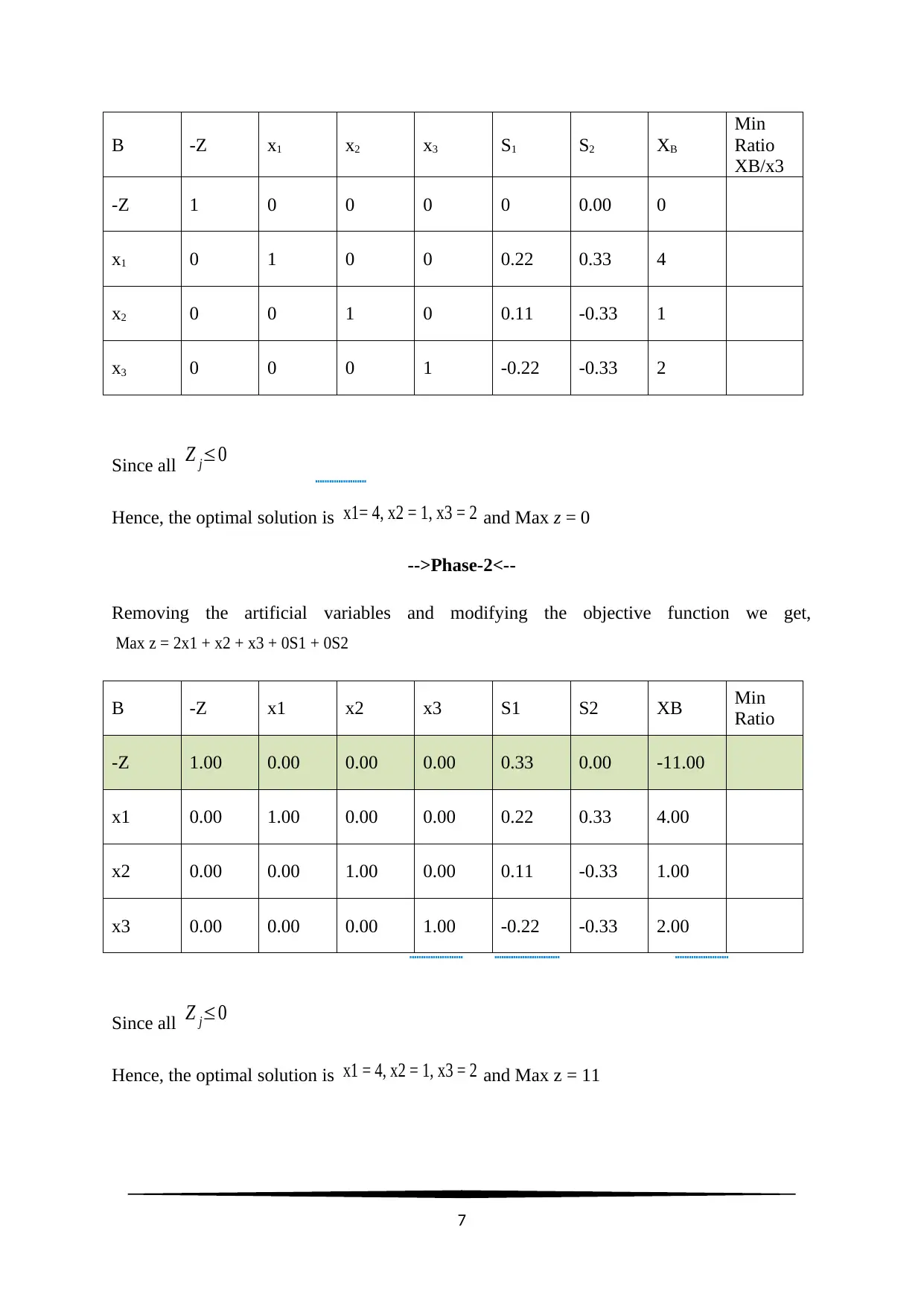
B -Z x1 x2 x3 S1 S2 XB
Min
Ratio
XB/x3
-Z 1 0 0 0 0 0.00 0
x1 0 1 0 0 0.22 0.33 4
x2 0 0 1 0 0.11 -0.33 1
x3 0 0 0 1 -0.22 -0.33 2
Since all Z j≤0
Hence, the optimal solution is x1= 4, x2 = 1, x3 = 2 and Max z = 0
-->Phase-2<--
Removing the artificial variables and modifying the objective function we get,
Max z = 2x1 + x2 + x3 + 0S1 + 0S2
B -Z x1 x2 x3 S1 S2 XB Min
Ratio
-Z 1.00 0.00 0.00 0.00 0.33 0.00 -11.00
x1 0.00 1.00 0.00 0.00 0.22 0.33 4.00
x2 0.00 0.00 1.00 0.00 0.11 -0.33 1.00
x3 0.00 0.00 0.00 1.00 -0.22 -0.33 2.00
Since all Z j≤0
Hence, the optimal solution is x1 = 4, x2 = 1, x3 = 2 and Max z = 11
7

Problem C
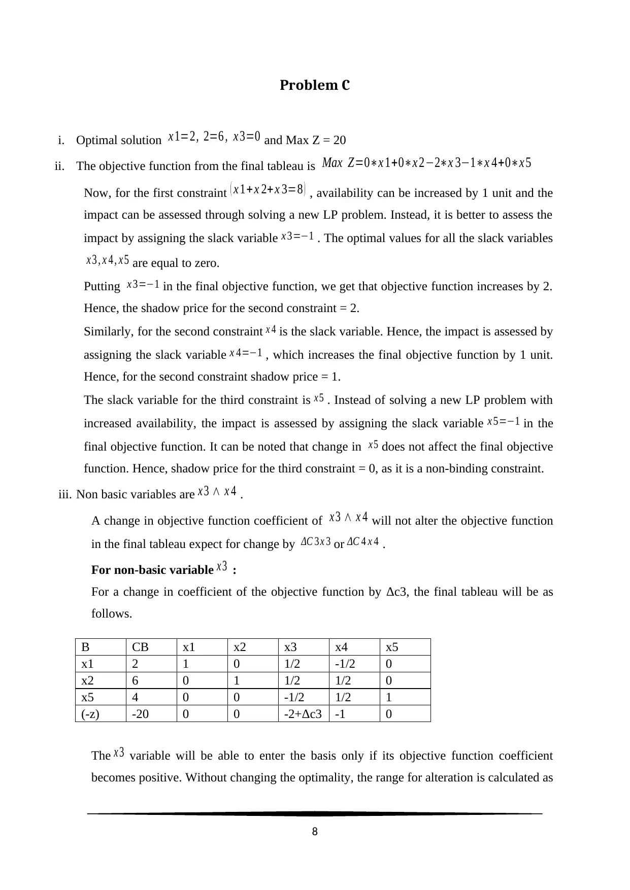
i. Optimal solution x 1=2, 2=6 , x 3=0 and Max Z = 20
ii. The objective function from the final tableau is Max Z=0∗x 1+0∗x 2−2∗x 3−1∗x 4+0∗x 5
Now, for the first constraint ( x 1+x 2+ x 3=8 ) , availability can be increased by 1 unit and the
impact can be assessed through solving a new LP problem. Instead, it is better to assess the
impact by assigning the slack variable x 3=−1 . The optimal values for all the slack variables
x 3 , x 4 , x 5 are equal to zero.
Putting x 3=−1 in the final objective function, we get that objective function increases by 2.
Hence, the shadow price for the second constraint = 2.
Similarly, for the second constraint x 4 is the slack variable. Hence, the impact is assessed by
assigning the slack variable x 4=−1 , which increases the final objective function by 1 unit.
Hence, for the second constraint shadow price = 1.
The slack variable for the third constraint is x 5 . Instead of solving a new LP problem with
increased availability, the impact is assessed by assigning the slack variable x 5=−1 in the
final objective function. It can be noted that change in x 5 does not affect the final objective
function. Hence, shadow price for the third constraint = 0, as it is a non-binding constraint.
iii. Non basic variables are x 3 ∧ x 4 .
A change in objective function coefficient of x 3 ∧ x 4 will not alter the objective function
in the final tableau expect for change by ΔC 3 x 3 or ΔC 4 x 4 .
For non-basic variable x 3 :
For a change in coefficient of the objective function by Δc3, the final tableau will be as
follows.
B CB x1 x2 x3 x4 x5
x1 2 1 0 1/2 -1/2 0
x2 6 0 1 1/2 1/2 0
x5 4 0 0 -1/2 1/2 1
(-z) -20 0 0 -2+Δc3 -1 0
The x 3 variable will be able to enter the basis only if its objective function coefficient
becomes positive. Without changing the optimality, the range for alteration is calculated as
8

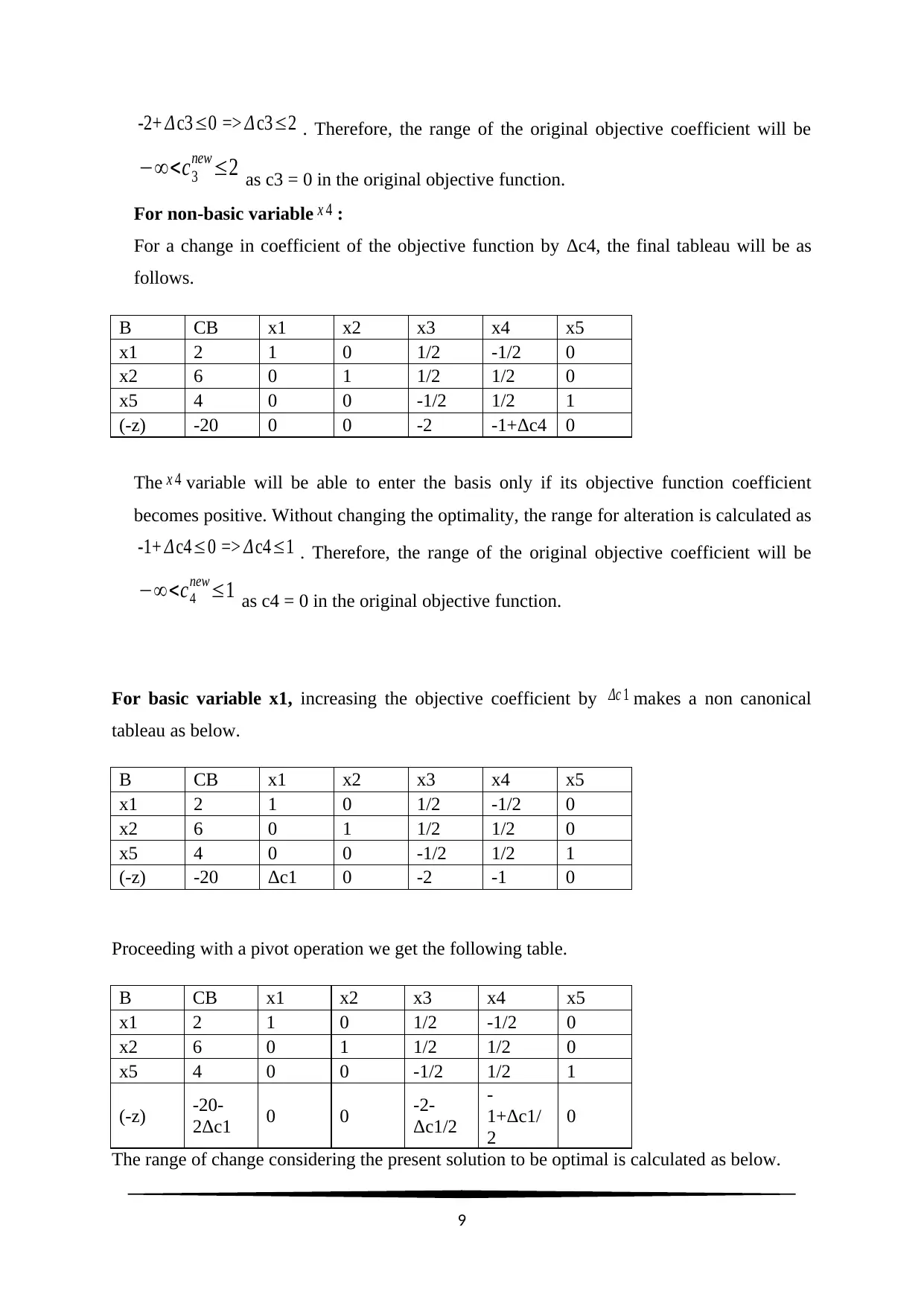
-2+ Δc3≤0 => Δ c3≤2 . Therefore, the range of the original objective coefficient will be
−∞<c3
new≤2 as c3 = 0 in the original objective function.
For non-basic variable x 4 :
For a change in coefficient of the objective function by Δc4, the final tableau will be as
follows.
B CB x1 x2 x3 x4 x5
x1 2 1 0 1/2 -1/2 0
x2 6 0 1 1/2 1/2 0
x5 4 0 0 -1/2 1/2 1
(-z) -20 0 0 -2 -1+Δc4 0
The x 4 variable will be able to enter the basis only if its objective function coefficient
becomes positive. Without changing the optimality, the range for alteration is calculated as
-1+ Δ c4≤0 => Δ c4≤1 . Therefore, the range of the original objective coefficient will be
−∞<c4
new≤1 as c4 = 0 in the original objective function.
For basic variable x1, increasing the objective coefficient by Δc 1 makes a non canonical
tableau as below.
B CB x1 x2 x3 x4 x5
x1 2 1 0 1/2 -1/2 0
x2 6 0 1 1/2 1/2 0
x5 4 0 0 -1/2 1/2 1
(-z) -20 Δc1 0 -2 -1 0
Proceeding with a pivot operation we get the following table.
B CB x1 x2 x3 x4 x5
x1 2 1 0 1/2 -1/2 0
x2 6 0 1 1/2 1/2 0
x5 4 0 0 -1/2 1/2 1
(-z) -20-
2Δc1 0 0 -2-
Δc1/2
-
1+Δc1/
2
0
The range of change considering the present solution to be optimal is calculated as below.
9

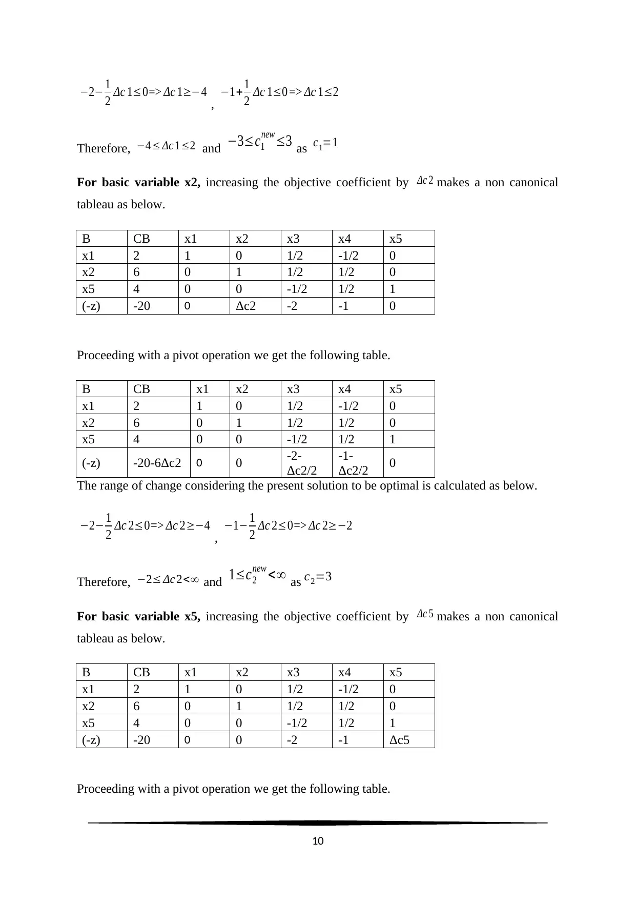
−2− 1
2 Δc 1≤0=> Δc 1≥−4 , −1+ 1
2 Δc 1≤0 => Δc 1≤2
Therefore, −4≤ Δc 1≤2 and −3≤c1
new≤3 as c1=1
For basic variable x2, increasing the objective coefficient by Δc 2 makes a non canonical
tableau as below.
B CB x1 x2 x3 x4 x5
x1 2 1 0 1/2 -1/2 0
x2 6 0 1 1/2 1/2 0
x5 4 0 0 -1/2 1/2 1
(-z) -20 0 Δc2 -2 -1 0
Proceeding with a pivot operation we get the following table.
B CB x1 x2 x3 x4 x5
x1 2 1 0 1/2 -1/2 0
x2 6 0 1 1/2 1/2 0
x5 4 0 0 -1/2 1/2 1
(-z) -20-6Δc2 0 0 -2-
Δc2/2
-1-
Δc2/2 0
The range of change considering the present solution to be optimal is calculated as below.
−2− 1
2 Δc 2≤0=> Δc 2≥−4 , −1− 1
2 Δc 2≤0=> Δc 2≥−2
Therefore, −2≤ Δc 2<∞ and 1≤c2
new <∞ as c2=3
For basic variable x5, increasing the objective coefficient by Δc 5 makes a non canonical
tableau as below.
B CB x1 x2 x3 x4 x5
x1 2 1 0 1/2 -1/2 0
x2 6 0 1 1/2 1/2 0
x5 4 0 0 -1/2 1/2 1
(-z) -20 0 0 -2 -1 Δc5
Proceeding with a pivot operation we get the following table.
10

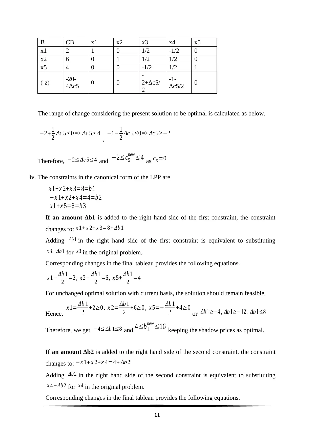
B CB x1 x2 x3 x4 x5
x1 2 1 0 1/2 -1/2 0
x2 6 0 1 1/2 1/2 0
x5 4 0 0 -1/2 1/2 1
(-z) -20-
4Δc5 0 0
-
2+Δc5/
2
-1-
Δc5/2 0
The range of change considering the present solution to be optimal is calculated as below.
−2+1
2 Δc 5≤0 => Δc 5≤4 , −1− 1
2 Δc 5≤0 => Δc5≥−2
Therefore, −2≤ Δc5≤4 and −2≤c5
new≤4 as c5=0
iv. The constraints in the canonical form of the LPP are
x 1+ x 2+ x 3=8=b 1
−x 1+ x 2+ x 4=4=b 2
x 1+ x 5=6=b 3
If an amount ∆b1 is added to the right hand side of the first constraint, the constraint
changes to: x 1+ x 2+ x 3=8+ Δb 1
Adding Δb 1 in the right hand side of the first constraint is equivalent to substituting
x 3−Δb 1 for x 3 in the original problem.
Corresponding changes in the final tableau provides the following equations.
x 1− Δb 1
2 =2 , x 2− Δb 1
2 =6 , x 5+ Δb1
2 =4
For unchanged optimal solution with current basis, the solution should remain feasible.
Hence, x 1= Δb 1
2 +2≥0 , x 2= Δb 1
2 +6≥0 , x 5=− Δb1
2 +4≥0 or Δb 1≥−4 , Δb 1≥−12, Δb 1≤8
Therefore, we get −4≤ Δb 1≤8 and 4≤b1
new≤16 keeping the shadow prices as optimal.
If an amount ∆b2 is added to the right hand side of the second constraint, the constraint
changes to: −x 1+ x 2+ x 4=4+ Δb 2
Adding Δb 2 in the right hand side of the second constraint is equivalent to substituting
x 4−Δb 2 for x 4 in the original problem.
Corresponding changes in the final tableau provides the following equations.
11

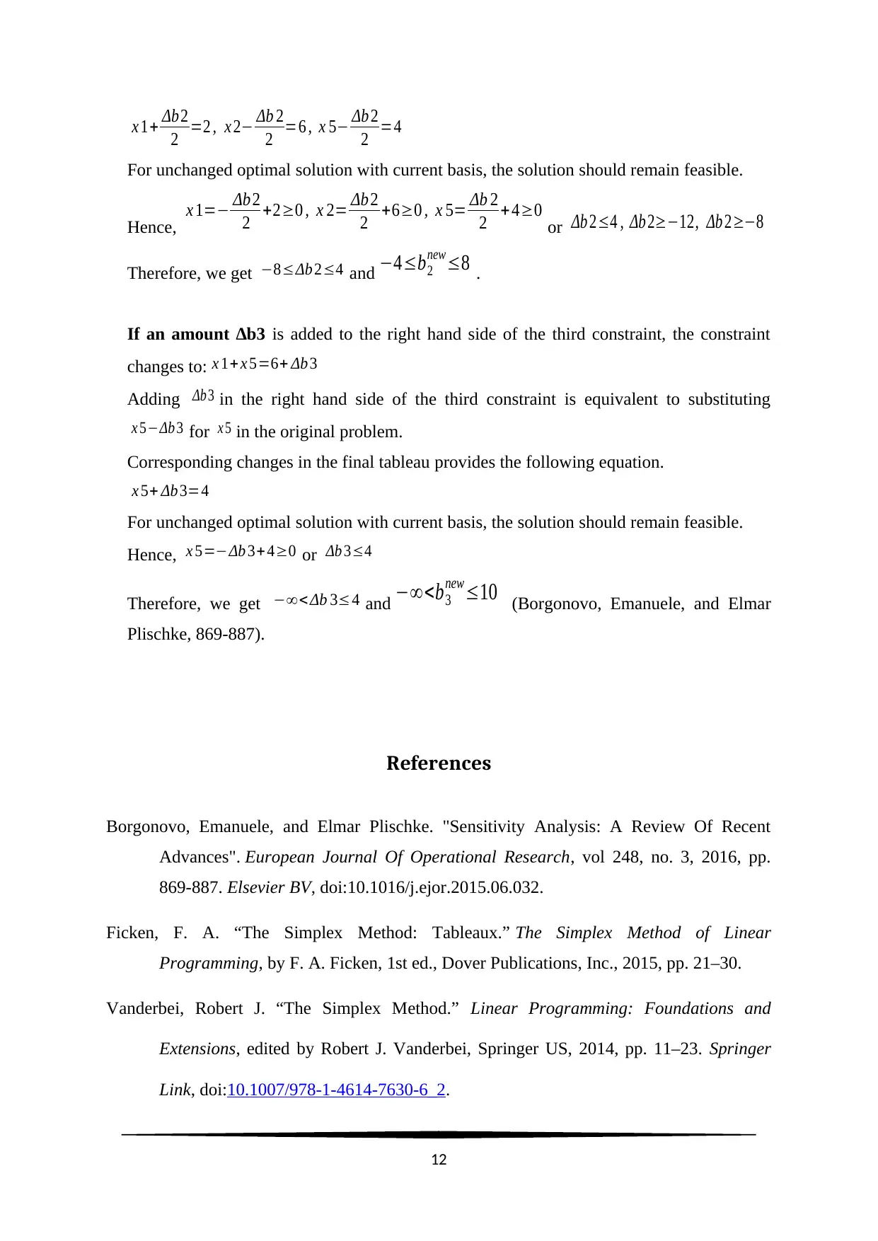
x 1+ Δb2
2 =2 , x 2− Δb 2
2 =6 , x 5− Δb 2
2 =4
For unchanged optimal solution with current basis, the solution should remain feasible.
Hence, x 1=− Δb2
2 +2≥0 , x 2= Δb2
2 +6≥0 , x 5= Δb 2
2 + 4≥0 or Δb 2≤4 , Δb2≥−12, Δb 2≥−8
Therefore, we get −8≤Δb 2≤4 and −4≤b2
new≤8 .
If an amount ∆b3 is added to the right hand side of the third constraint, the constraint
changes to: x 1+ x 5=6+ Δb 3
Adding Δb3 in the right hand side of the third constraint is equivalent to substituting
x 5−Δb 3 for x 5 in the original problem.
Corresponding changes in the final tableau provides the following equation.
x 5+ Δb 3=4
For unchanged optimal solution with current basis, the solution should remain feasible.
Hence, x 5=−Δb 3+ 4≥0 or Δb 3≤4
Therefore, we get −∞< Δb 3≤4 and −∞<b3
new≤10 (Borgonovo, Emanuele, and Elmar
Plischke, 869-887).
References
Borgonovo, Emanuele, and Elmar Plischke. "Sensitivity Analysis: A Review Of Recent
Advances". European Journal Of Operational Research, vol 248, no. 3, 2016, pp.
869-887. Elsevier BV, doi:10.1016/j.ejor.2015.06.032.
Ficken, F. A. “The Simplex Method: Tableaux.” The Simplex Method of Linear
Programming, by F. A. Ficken, 1st ed., Dover Publications, Inc., 2015, pp. 21–30.
Vanderbei, Robert J. “The Simplex Method.” Linear Programming: Foundations and
Extensions, edited by Robert J. Vanderbei, Springer US, 2014, pp. 11–23. Springer
Link, doi:10.1007/978-1-4614-7630-6_2.
12