Linear Regression and Correlation Analysis in R: ADMISSION Assignment

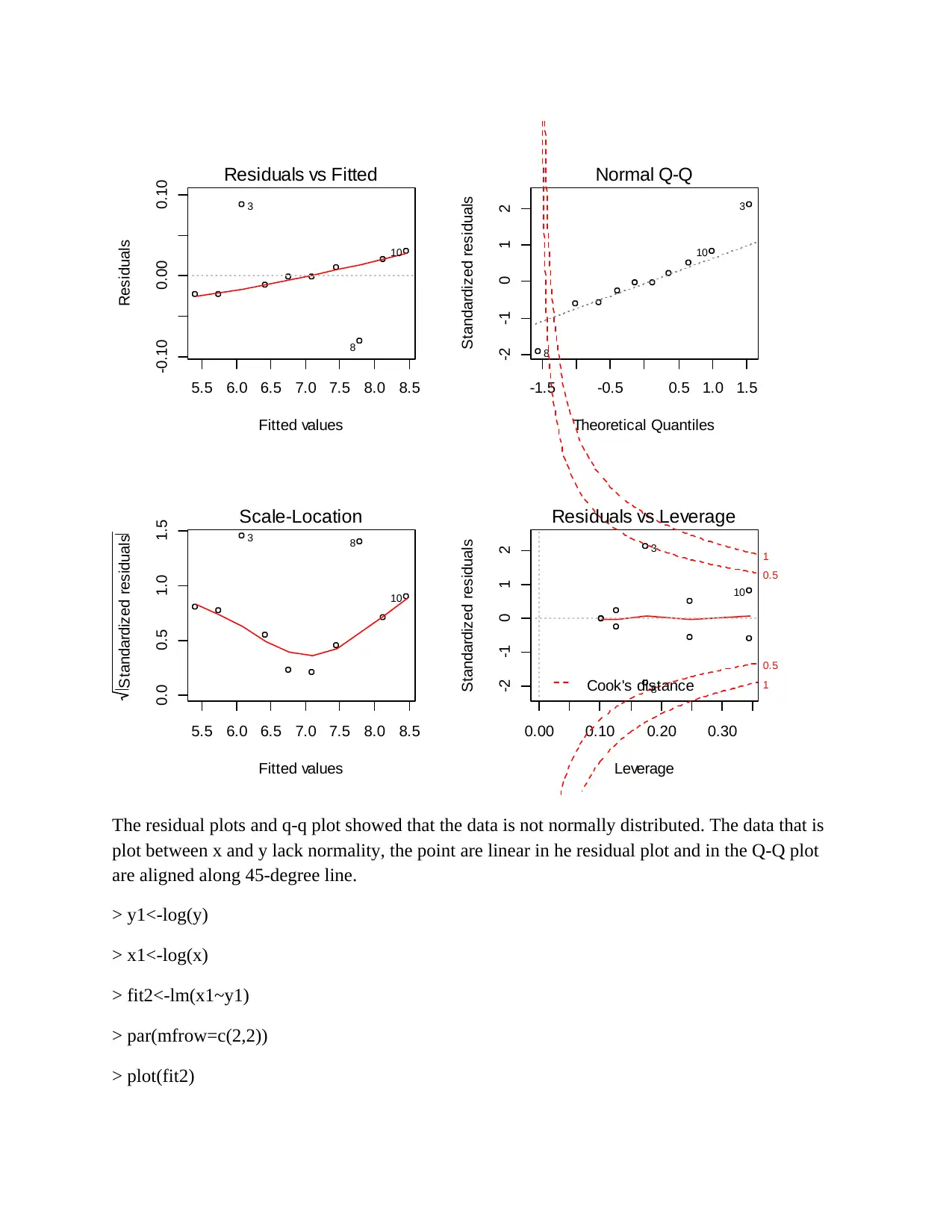
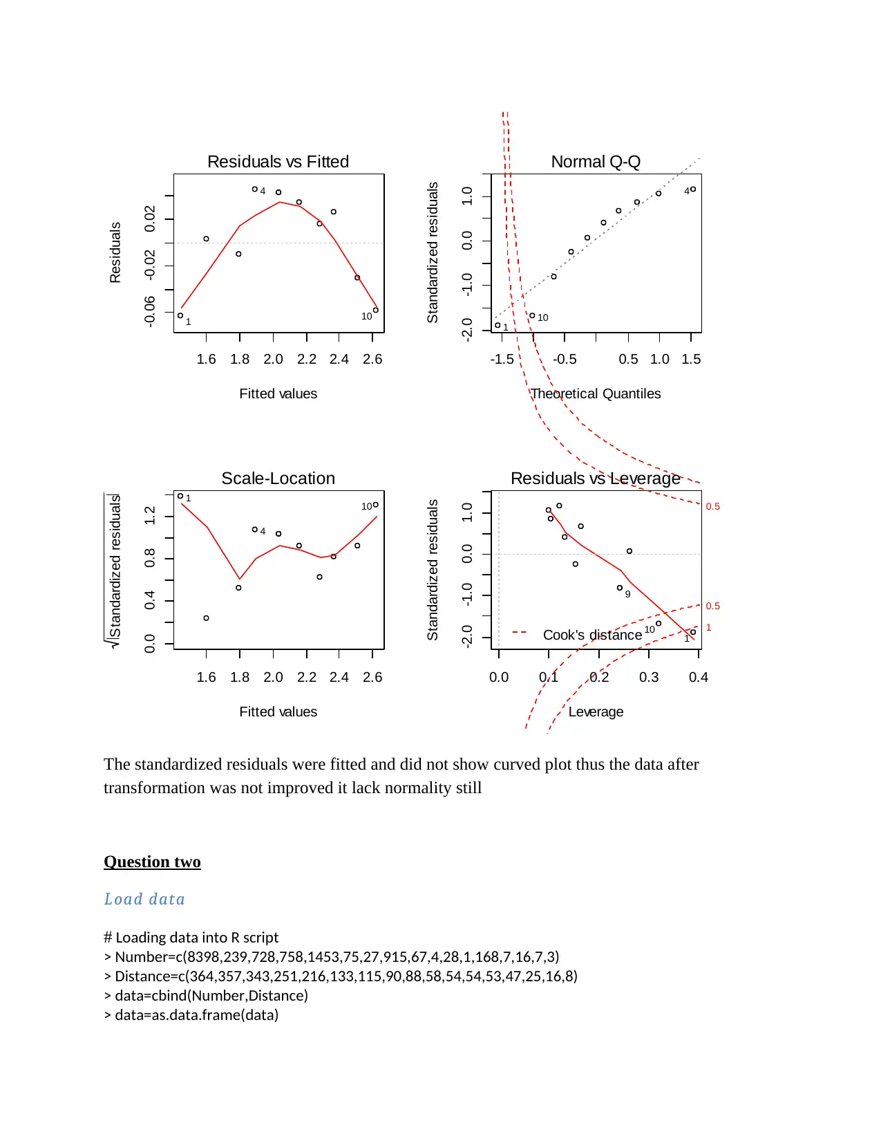
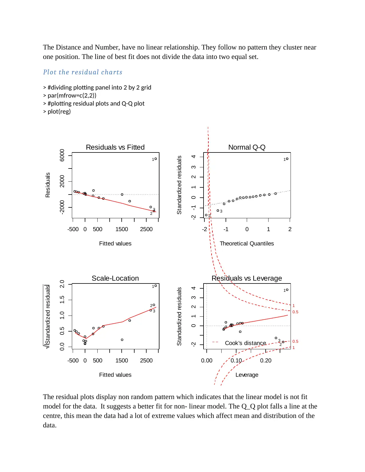
This assignment demonstrates linear regression and correlation analysis using the R programming language. The solution begins by loading data and calculating linear regression models, including interpreting coefficients, p-values, and R-squared values. The analysis involves creating scatter plots and residual plots to assess model fit and identify potential issues like non-normality and non-linearity. The assignment then explores data transformation techniques, specifically logarithmic transformations, to improve model fit and address violations of assumptions. Two distinct datasets are analyzed, with the second dataset focusing on the relationship between 'Number' and 'Distance'. The solution includes model fitting, interpretation of results, and an evaluation of the impact of data transformation on model performance. The student explores the use of scatter plots, residual plots, and Q-Q plots to diagnose the model's performance, including the normality of the data, and the linearity. The assignment concludes by analyzing the impact of data transformation on the model's fit and interpretation.

ASSIGNMENT
Linear Regression and Correlation Analysis in R
NAME:
COURSE:
ADMISSION:
Question One
Load data
#loading the data in R script window
>y=c(5.39,5.73,6.18,6.42,6.77,7.11,7.46,7.71,8.15,8.5)
>x=c(4,5,6,7,8,9,10,11,12,13)
>dat=cbind(x,y)
>dat=as.data.frame(dat
Calculate the linear regression (Distance is predictor variable, Number is
response variable)

>#regression modelling
>fit<-lm(y~x)
#output of the model
>fit
Call:
lm(formula = y ~ x)
Coefficients:
(Intercept) x
4.0551 0.3396
 The equation of the line Y=4.0551+ 0.3396 x
> #obtaining summary of of statistics
> summary(fit)
Call:
lm(formula = y ~ x)
Residuals:
Min 1Q Median 3Q Max
-0.08109 -0.02059 -0.00200 0.01659 0.08709
Coefficients:
Estimate Std. Error t value Pr(>|t|)
(Intercept) 4.055091 0.045198 89.72 2.66e-13 ***
x 0.339636 0.005038 67.42 2.61e-12 ***

---
Signif. codes: 0 ‘***’ 0.001 ‘**’ 0.01 ‘*’ 0.05 ‘.’ 0.1 ‘ ’ 1
Residual standard error: 0.04576 on 8 degrees of freedom
Multiple R-squared: 0.9982, Adjusted R-squared: 0.998
F-statistic: 4545 on 1 and 8 DF, p-value: 2.607e-12
 The null hypothesis is predictor variable (x) is not significance in the model. The p-value
is 2.607e-12 which is less than the level of significance 0.05 therefore we reject the null
hypothesis and conclude that the predictor variable (x) is significance in the model. It can
be used to predict response variable (y).
 The R-squared is 0.9982 which means 99.82% of the variation in y are explained by x
thus the model is good fit
Plot the best fit line on a scatterplot of the data
>#ploting the scatterplot
>plot(x,y, abline(fit), main="Scatter plot")

4 6 8 10 12
5.5 6.0 6.5 7.0 7.5 8.0 8.5
Scatter plot
x
y
The relation between x and y is positive linear. Only few points which lies outside the line of
best fit.
Plot the residual charts
> #split the plotting panel into 2 times 2 grid
> par(mfrow=c(2,2))
> #residuals plotting
> plot(fit)

5.5 6.0 6.5 7.0 7.5 8.0 8.5
-0.10 0.00 0.10
Fitted values
Residuals
Residuals vs Fitted
3
8
10
-1.5 -0.5 0.5 1.0 1.5
-2 -1 0 1 2
Theoretical Quantiles
Standardized residuals
Normal Q-Q
3
8
10
5.5 6.0 6.5 7.0 7.5 8.0 8.5
0.0 0.5 1.0 1.5
Fitted values
Standardized residuals Scale-Location
3 8
10
0.00 0.10 0.20 0.30
-2 -1 0 1 2
Leverage
Standardized residuals
Cook's distance 1
0.5
0.5
1
Residuals vs Leverage
3
8
10
The residual plots and q-q plot showed that the data is not normally distributed. The data that is
plot between x and y lack normality, the point are linear in he residual plot and in the Q-Q plot
are aligned along 45-degree line.
> y1<-log(y)
> x1<-log(x)
> fit2<-lm(x1~y1)
> par(mfrow=c(2,2))
> plot(fit2)

1.6 1.8 2.0 2.2 2.4 2.6
-0.06 -0.02 0.02
Fitted values
Residuals
Residuals vs Fitted
1 10
4
-1.5 -0.5 0.5 1.0 1.5
-2.0 -1.0 0.0 1.0
Theoretical Quantiles
Standardized residuals
Normal Q-Q
1 10
4
1.6 1.8 2.0 2.2 2.4 2.6
0.0 0.4 0.8 1.2
Fitted values
Standardized residuals Scale-Location
1 10
4
0.0 0.1 0.2 0.3 0.4
-2.0 -1.0 0.0 1.0
Leverage
Standardized residuals
Cook's distance 1
0.5
0.5
Residuals vs Leverage
1
10
9
The standardized residuals were fitted and did not show curved plot thus the data after
transformation was not improved it lack normality still
Question two
Load data
# Loading data into R script
> Number=c(8398,239,728,758,1453,75,27,915,67,4,28,1,168,7,16,7,3)
> Distance=c(364,357,343,251,216,133,115,90,88,58,54,54,53,47,25,16,8)
> data=cbind(Number,Distance)
> data=as.data.frame(data)

Calculate the linear regression (Distance is predictor variable, Number is
response variable)
> #fitting the model
> reg<-lm(Number~Distance)
> #calling the model
> reg
Call:
lm(formula = Number ~ Distance)
Coefficients:
(Intercept) Distance
-485.699 9.309
 The regression model is Number=−485.699+ 9.309 Distance
 The null hypothesis is distance is not significance in Number=−485.699+ 9.309 Distance
model. The p-value is 0.0163 and the level of significance is 0.01, which is greater than
the level of significance. Thus we fail to reject null hypothesis and conclude that distance
is not significance in predicting number and can be dropped from the model.
> summary(reg)
Call:
lm(formula = Number ~ Distance)
Residuals:
Min 1Q Median 3Q Max
-2598.7 -557.9 -16.0 269.0 5495.1
Coefficients:
Estimate Std. Error t value Pr(>|t|)
(Intercept) -485.699 618.551 -0.785 0.4446
Distance 9.309 3.441 2.705 0.0163 *

---
Signif. codes: 0 ‘***’ 0.001 ‘**’ 0.01 ‘*’ 0.05 ‘.’ 0.1 ‘ ’ 1
Residual standard error: 1705 on 15 degrees of freedom
Multiple R-squared: 0.3279, Adjusted R-squared: 0.2831
F-statistic: 7.317 on 1 and 15 DF, p-value: 0.01629
 R-squared is 0.3279 which means only 32.79% variations in distance are explained by
distance. The model is poor fit and distance can not be used to predict number.
Plot the best fit line on a scatterplot of the data
> #plotting scatter plot of distance vs number and imposing a line of best fit
> plot(Distance, Number, abline(reg), main="Scatter plot of Distance Vs Number")
0 50 100 150 200 250 300 350
0 2000 4000 6000 8000
Scatter plot of Distance Vs Number
Distance
Number

The Distance and Number, have no linear relationship. They follow no pattern they cluster near
one position. The line of best fit does not divide the data into two equal set.
Plot the residual charts
> #dividing plotting panel into 2 by 2 grid
> par(mfrow=c(2,2))
> #plotting residual plots and Q-Q plot
> plot(reg)
-500 0 500 1500 2500
-2000 2000 6000
Fitted values
Residuals
Residuals vs Fitted
1
2 3
-2 -1 0 1 2
-2 -1 0 1 2 3 4
Theoretical Quantiles
Standardized residuals
Normal Q-Q
1
2
3
-500 0 500 1500 2500
0.0 0.5 1.0 1.5 2.0
Fitted values
Standardized residuals Scale-Location 1
2
3
0.00 0.10 0.20
-2 0 1 2 3 4
Leverage
Standardized residuals
Cook's distance 1
0.5
0.5
1
Residuals vs Leverage
1
2
3
The residual plots display non random pattern which indicates that the linear model is not fit
model for the data. It suggests a better fit for non- linear model. The Q_Q plot falls a line at the
centre, this mean the data had a lot of extreme values which affect mean and distribution of the
data.

Could you improve the model fit by transforming the data?
The data can be improved through transformation, the most common methods of transformation
is square root, squaring, inverse and log transformation.
> number1<-log(Number)
> distance1<-log(Distance)
> reg1<-lm(number1~distance1)
> reg1
Call:
lm(formula = number1 ~ distance1)
Coefficients:
(Intercept) distance1
-3.695 1.786
> summary(reg1)
Call:
lm(formula = number1 ~ distance1)
Residuals:
Min 1Q Median 3Q Max
-3.4305 -1.2366 -0.0982 1.0792 2.4759
Coefficients:

Estimate Std. Error t value Pr(>|t|)
(Intercept) -3.6953 1.6974 -2.177 0.045863 *
distance1 1.7864 0.3737 4.781 0.000243 ***
---
Signif. codes: 0 ‘***’ 0.001 ‘**’ 0.01 ‘*’ 0.05 ‘.’ 0.1 ‘ ’ 1
Residual standard error: 1.648 on 15 degrees of freedom
Multiple R-squared: 0.6038, Adjusted R-squared: 0.5773
F-statistic: 22.86 on 1 and 15 DF, p-value: 0.0002429
 The equation of transformation is log ¿er)=a+log ¿)
Number =−3.695+1.786 log ¿)
 The p-value 0.000243 which is less than level of significance of 0.05 so we reject null
hypothesis and conclude that distance is significance in predicting number.
 The R-squared is 0.6038 which implies that 60.38% of the responses are explained by the
predictor and the model is a good fit.
Scatter plot
> #scatter plot
> plot(distance1, number1, abline(reg), main="Scatter plot of Distance Vs Number")

2 3 4 5 6
0 2 4 6 8
Scatter plot of Distance Vs Number
distance1
number1
 The line of best fit sub divide the data into two equal parts thus the data is linear.
> #dividing plotting panel into 2 by 2 grid
> par(mfrow=c(2,2))
> #plotting residual plots and Q-Q plot
> plot(reg1)

0 1 2 3 4 5 6 7
-4 -2 0 1 2 3
Fitted values
Residuals
Residuals vs Fitted
12
8 1
-2 -1 0 1 2
-2 -1 0 1
Theoretical Quantiles
Standardized residuals
Normal Q-Q
12
81
0 1 2 3 4 5 6 7
0.0 0.5 1.0 1.5
Fitted values
Standardized residuals Scale-Location
12
8 1
0.00 0.10 0.20 0.30
-2 -1 0 1 2
Leverage
Standardized residuals
Cook's distance 1
0.5
0.5
1
Residuals vs Leverage
1
12
17
 The data displays u-shaped non random pattern. This suggests that linear model is not a
fit model for the data. The data is non linear model.
 The Q-Q plot follows a straight line which suggests that the data is from normal
distribution.
 The fitted value shows that the data is not from equal variance.
The transformation improved normality but not linearity. Even after transformation the
data is non – linear.