EECS 152B Winter 2019 Assignment 3 - LMS and RLS Noise Canceller
VerifiedAdded on 2023/04/21
|11
|2041
|354
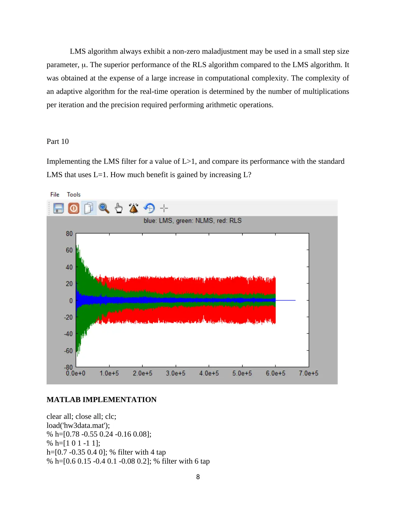
Homework Assignment
AI Summary
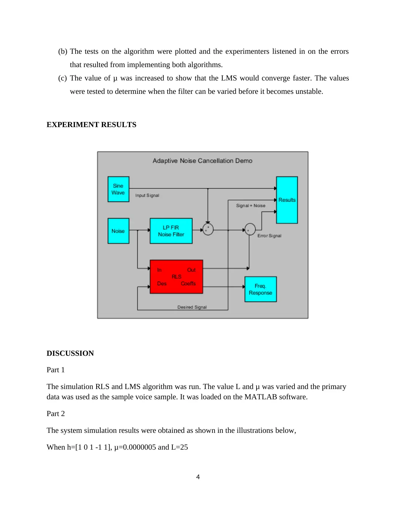
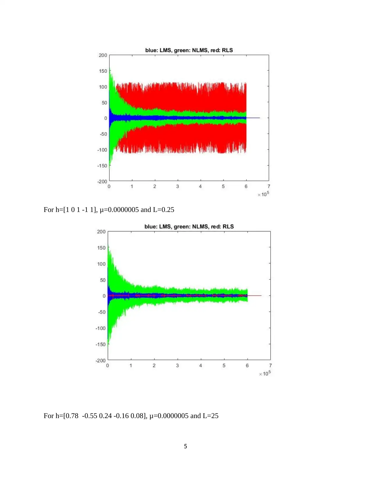
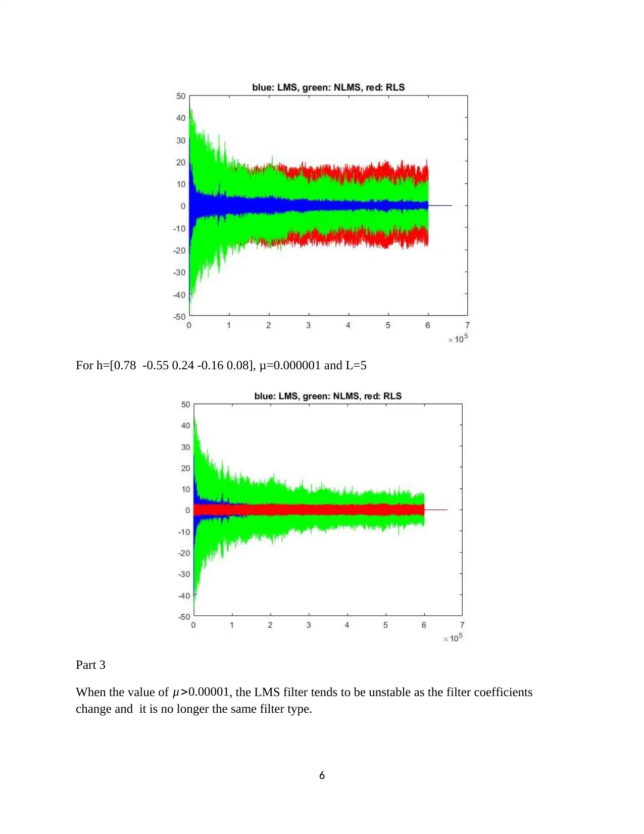
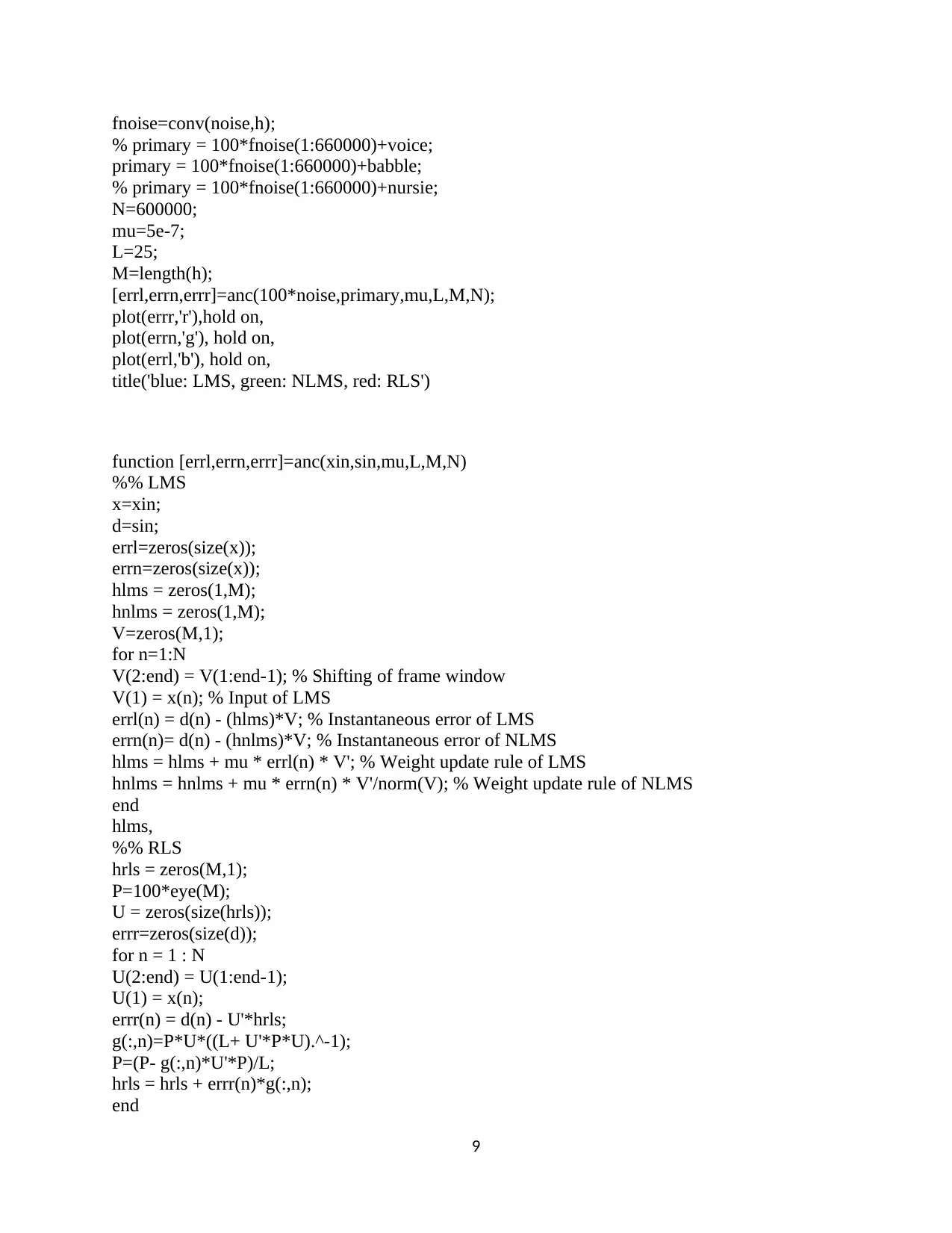
This assignment solution details the implementation of an adaptive noise canceller using the Least Mean Squares (LMS) and Recursive Least Squares (RLS) algorithms in MATLAB, as part of the EECS 152B Winter 2019 course. The experiment involves recovering a voice signal buried in noise by generating a filtered version of the reference noise and convolving it with an impulse response vector. The document covers the theoretical background, including the mathematical derivations of both algorithms, the experimental procedure, and a discussion of the results obtained by varying parameters such as µ and L. It further analyzes the stability and convergence properties of the LMS and RLS filters under different conditions, concluding with the MATLAB code used for the implementation and simulation of the adaptive noise cancellation system.

1 out of 11


Your All-in-One AI-Powered Toolkit for Academic Success.
+13062052269
info@desklib.com
Available 24*7 on WhatsApp / Email
![[object Object]](/_next/static/media/star-bottom.7253800d.svg)
Copyright © 2020–2026 A2Z Services. All Rights Reserved. Developed and managed by ZUCOL.