Logistic & Supply Chain Optimization Problem: Detailed Report
VerifiedAdded on 2023/06/09
|19
|4007
|233
Report
AI Summary
This document provides a detailed solution to an optimization problem in logistic and supply chain management. The problem involves optimizing recycling operations across 10 sectors and 5 recycling sites, considering factors such as capacity, efficiency, and transportation costs. The solution explores maximizing garbage consumption and minimizing costs using Excel Solver, including scenarios with tripled plant capacity and Multi-Objective Linear Programming (MOLP). Additionally, the document addresses a distance minimization problem for warehouse locations and discusses criteria for supplier selection. The analysis includes calculations, tables, and explanations of the optimization processes and results, with the aim of improving recycling efficiency and reducing operational costs.
Optimization problem
1 | P a g e
Logistic and Supply chain management
1 | P a g e
Logistic and Supply chain management
Paraphrase This Document
Need a fresh take? Get an instant paraphrase of this document with our AI Paraphraser
Optimization problem
Contents
Solution 1.........................................................................................................................................3
Solution1(a).................................................................................................................................3
Solution1(b).................................................................................................................................7
Solution1(c).................................................................................................................................8
Solution 2.........................................................................................................................................9
Solution 3.......................................................................................................................................10
Solution 4.......................................................................................................................................14
References......................................................................................................................................18
2 | P a g e
Optimization problem
Solution 1
Solution1(a)
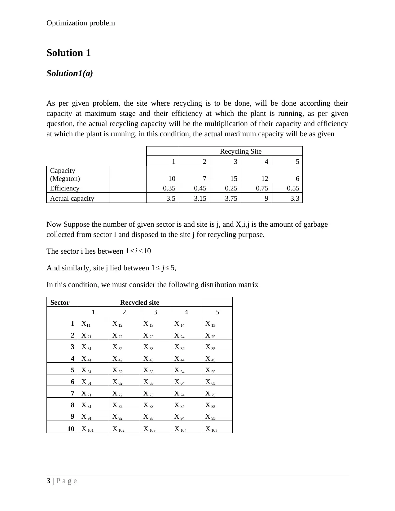
As per given problem, the site where recycling is to be done, will be done according their
capacity at maximum stage and their efficiency at which the plant is running, as per given
question, the actual recycling capacity will be the multiplication of their capacity and efficiency
at which the plant is running, in this condition, the actual maximum capacity will be as given
Recycling Site
1 2 3 4 5
Capacity
(Megaton) 10 7 15 12 6
Efficiency 0.35 0.45 0.25 0.75 0.55
Actual capacity 3.5 3.15 3.75 9 3.3
Now Suppose the number of given sector is and site is j, and X,i,j is the amount of garbage
collected from sector I and disposed to the site j for recycling purpose.
The sector i lies between 1 ≤i ≤10
And similarly, site j lied between 1 ≤ j≤ 5,
In this condition, we must consider the following distribution matrix
Sector Recycled site
1 2 3 4 5
1 X11 X 12 X 13 X 14 X 15
2 X 21 X 22 X 23 X 24 X 25
3 X 31 X 32 X 33 X 34 X 35
4 X 41 X 42 X 43 X 44 X 45
5 X 51 X 52 X 53 X 54 X 55
6 X 61 X 62 X 63 X 64 X 65
7 X 71 X 72 X 73 X 74 X 75
8 X 81 X 82 X 83 X 84 X 85
9 X 91 X 92 X 93 X 94 X 95
10 X 101 X 102 X 103 X 104 X 105
3 | P a g e
Solution 1
Solution1(a)
As per given problem, the site where recycling is to be done, will be done according their
capacity at maximum stage and their efficiency at which the plant is running, as per given
question, the actual recycling capacity will be the multiplication of their capacity and efficiency
at which the plant is running, in this condition, the actual maximum capacity will be as given
Recycling Site
1 2 3 4 5
Capacity
(Megaton) 10 7 15 12 6
Efficiency 0.35 0.45 0.25 0.75 0.55
Actual capacity 3.5 3.15 3.75 9 3.3
Now Suppose the number of given sector is and site is j, and X,i,j is the amount of garbage
collected from sector I and disposed to the site j for recycling purpose.
The sector i lies between 1 ≤i ≤10
And similarly, site j lied between 1 ≤ j≤ 5,
In this condition, we must consider the following distribution matrix
Sector Recycled site
1 2 3 4 5
1 X11 X 12 X 13 X 14 X 15
2 X 21 X 22 X 23 X 24 X 25
3 X 31 X 32 X 33 X 34 X 35
4 X 41 X 42 X 43 X 44 X 45
5 X 51 X 52 X 53 X 54 X 55
6 X 61 X 62 X 63 X 64 X 65
7 X 71 X 72 X 73 X 74 X 75
8 X 81 X 82 X 83 X 84 X 85
9 X 91 X 92 X 93 X 94 X 95
10 X 101 X 102 X 103 X 104 X 105
3 | P a g e
⊘ This is a preview!⊘
Do you want full access?
Subscribe today to unlock all pages.
Trusted by 1+ million students worldwide
Optimization problem
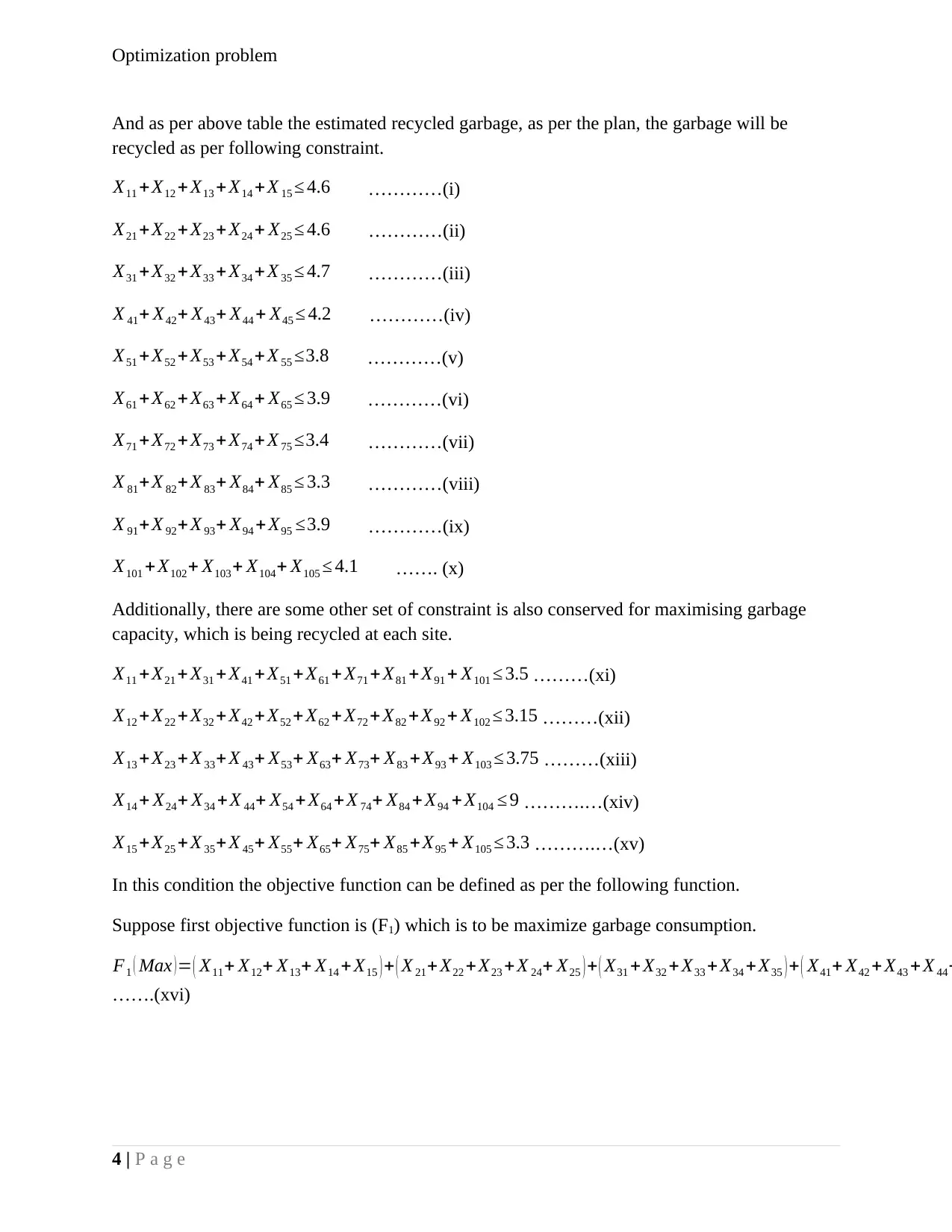
And as per above table the estimated recycled garbage, as per the plan, the garbage will be
recycled as per following constraint.
X11 +X12 + X13 + X14 +X 15 ≤ 4.6 …………(i)
X21 + X22 + X23 +X24 + X25 ≤ 4.6 …………(ii)
X31 + X32 + X33 +X34 + X 35 ≤ 4.7 …………(iii)
X 41+ X42+ X43+ X44 + X45 ≤ 4.2 …………(iv)
X51 + X52 + X53 +X54 + X 55 ≤3.8 …………(v)
X61 + X62 + X63 +X64 + X65 ≤ 3.9 …………(vi)
X71 + X72 + X73 +X74 + X 75 ≤3.4 …………(vii)
X 81+ X 82+ X 83+ X84+ X85 ≤ 3.3 …………(viii)
X 91+ X 92+ X 93+ X94 + X95 ≤3.9 …………(ix)
X101 + X102+ X103+ X104+ X105 ≤ 4.1 ……. (x)
Additionally, there are some other set of constraint is also conserved for maximising garbage
capacity, which is being recycled at each site.
X11 +X21 + X31 +X41 + X51 +X61 + X71 + X81 + X91 + X101 ≤ 3.5 ………(xi)
X12 + X22 + X32 +X42 + X52 + X62 +X72 + X82 + X92 + X102 ≤ 3.15 ………(xii)
X13 + X23 + X 33+X 43+ X53+ X63+ X73+ X83 +X93 + X103 ≤ 3.75 ………(xiii)
X14 + X24+ X34 + X 44+ X54 +X64 +X 74+ X84 +X94 + X104 ≤ 9 ……….…(xiv)
X15 + X25 + X 35+X 45+ X55+ X65+ X75+ X85 +X95 + X105 ≤ 3.3 ……….…(xv)
In this condition the objective function can be defined as per the following function.
Suppose first objective function is (F1) which is to be maximize garbage consumption.
F1 ( Max )= ( X11+ X12+ X13+ X14 + X15 ) + ( X 21+ X22 +X23 +X 24+ X25 ) + ( X31 + X32 + X33 + X34 +X35 ) + ( X41+ X42 + X43 + X 44+
…….(xvi)
4 | P a g e
Paraphrase This Document
Need a fresh take? Get an instant paraphrase of this document with our AI Paraphraser
Optimization problem
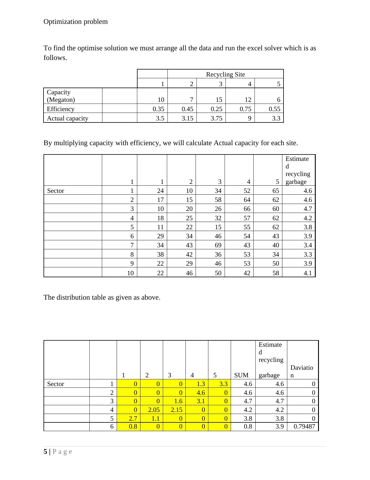
To find the optimise solution we must arrange all the data and run the excel solver which is as
follows.
Recycling Site
1 2 3 4 5
Capacity
(Megaton) 10 7 15 12 6
Efficiency 0.35 0.45 0.25 0.75 0.55
Actual capacity 3.5 3.15 3.75 9 3.3
By multiplying capacity with efficiency, we will calculate Actual capacity for each site.
1 1 2 3 4 5
Estimate
d
recycling
garbage
Sector 1 24 10 34 52 65 4.6
2 17 15 58 64 62 4.6
3 10 20 26 66 60 4.7
4 18 25 32 57 62 4.2
5 11 22 15 55 62 3.8
6 29 34 46 54 43 3.9
7 34 43 69 43 40 3.4
8 38 42 36 53 34 3.3
9 22 29 46 53 50 3.9
10 22 46 50 42 58 4.1
The distribution table as given as above.
1 2 3 4 5 SUM
Estimate
d
recycling
garbage
Daviatio
n
Sector 1 0 0 0 1.3 3.3 4.6 4.6 0
2 0 0 0 4.6 0 4.6 4.6 0
3 0 0 1.6 3.1 0 4.7 4.7 0
4 0 2.05 2.15 0 0 4.2 4.2 0
5 2.7 1.1 0 0 0 3.8 3.8 0
6 0.8 0 0 0 0 0.8 3.9 0.79487
5 | P a g e
Optimization problem
2
7 0 0 0 0 0 0 3.4 1
8 0 0 0 0 0 0 3.3 1
9 0 0 0 0 0 0 3.9 1
10 0 0 0 0 0 0 4.1 1
SUM 3.5 3.15 3.75 9 3.3
0.47948
7
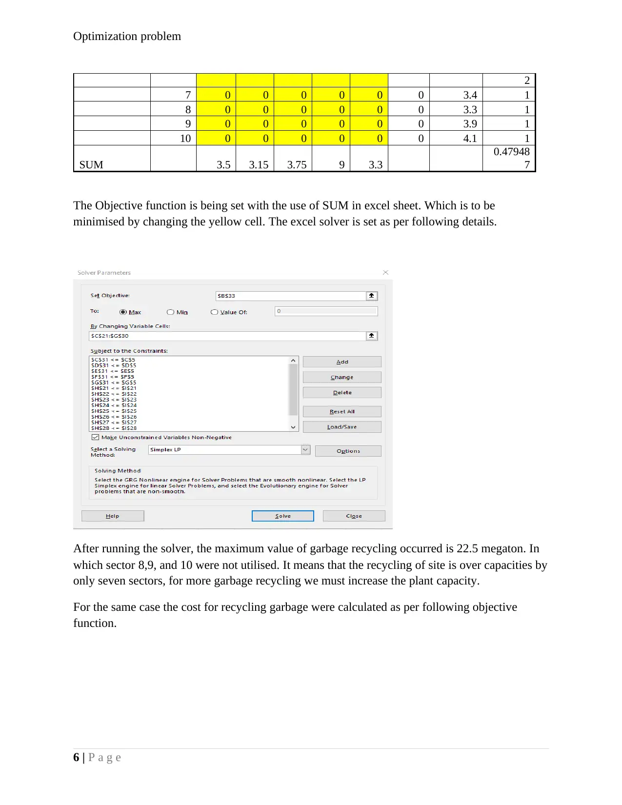
The Objective function is being set with the use of SUM in excel sheet. Which is to be
minimised by changing the yellow cell. The excel solver is set as per following details.
After running the solver, the maximum value of garbage recycling occurred is 22.5 megaton. In
which sector 8,9, and 10 were not utilised. It means that the recycling of site is over capacities by
only seven sectors, for more garbage recycling we must increase the plant capacity.
For the same case the cost for recycling garbage were calculated as per following objective
function.
6 | P a g e
2
7 0 0 0 0 0 0 3.4 1
8 0 0 0 0 0 0 3.3 1
9 0 0 0 0 0 0 3.9 1
10 0 0 0 0 0 0 4.1 1
SUM 3.5 3.15 3.75 9 3.3
0.47948
7
The Objective function is being set with the use of SUM in excel sheet. Which is to be
minimised by changing the yellow cell. The excel solver is set as per following details.
After running the solver, the maximum value of garbage recycling occurred is 22.5 megaton. In
which sector 8,9, and 10 were not utilised. It means that the recycling of site is over capacities by
only seven sectors, for more garbage recycling we must increase the plant capacity.
For the same case the cost for recycling garbage were calculated as per following objective
function.
6 | P a g e
⊘ This is a preview!⊘
Do you want full access?
Subscribe today to unlock all pages.
Trusted by 1+ million students worldwide
Optimization problem
Solution1(b)
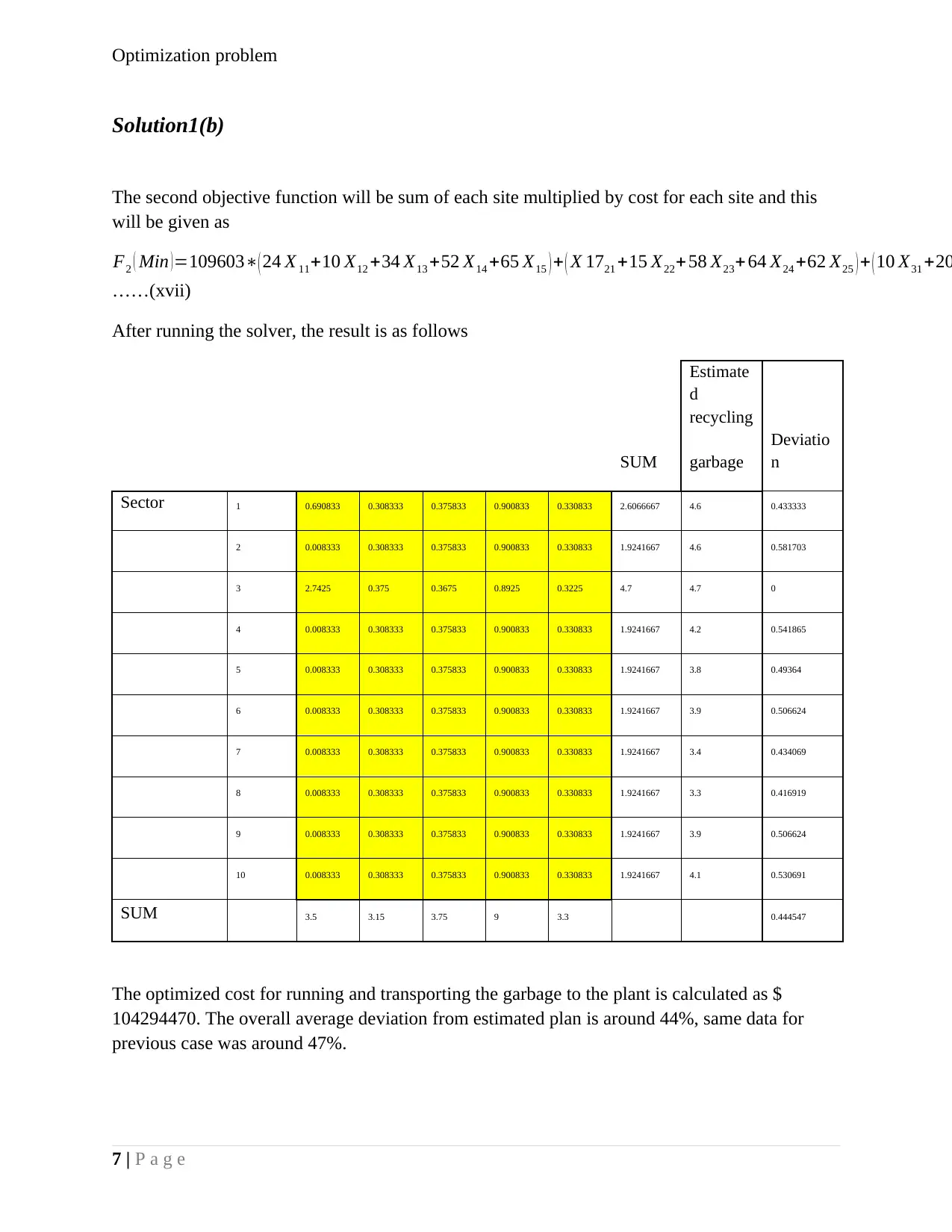
The second objective function will be sum of each site multiplied by cost for each site and this
will be given as
F2 ( Min ) =109603∗( 24 X 11+10 X12 +34 X13 +52 X14 +65 X15 ) + ( X 1721 +15 X22+ 58 X23+ 64 X24 +62 X25 ) + ( 10 X31 +20
……(xvii)
After running the solver, the result is as follows
SUM
Estimate
d
recycling
garbage
Deviatio
n
Sector 1 0.690833 0.308333 0.375833 0.900833 0.330833 2.6066667 4.6 0.433333
2 0.008333 0.308333 0.375833 0.900833 0.330833 1.9241667 4.6 0.581703
3 2.7425 0.375 0.3675 0.8925 0.3225 4.7 4.7 0
4 0.008333 0.308333 0.375833 0.900833 0.330833 1.9241667 4.2 0.541865
5 0.008333 0.308333 0.375833 0.900833 0.330833 1.9241667 3.8 0.49364
6 0.008333 0.308333 0.375833 0.900833 0.330833 1.9241667 3.9 0.506624
7 0.008333 0.308333 0.375833 0.900833 0.330833 1.9241667 3.4 0.434069
8 0.008333 0.308333 0.375833 0.900833 0.330833 1.9241667 3.3 0.416919
9 0.008333 0.308333 0.375833 0.900833 0.330833 1.9241667 3.9 0.506624
10 0.008333 0.308333 0.375833 0.900833 0.330833 1.9241667 4.1 0.530691
SUM 3.5 3.15 3.75 9 3.3 0.444547
The optimized cost for running and transporting the garbage to the plant is calculated as $
104294470. The overall average deviation from estimated plan is around 44%, same data for
previous case was around 47%.
7 | P a g e
Solution1(b)
The second objective function will be sum of each site multiplied by cost for each site and this
will be given as
F2 ( Min ) =109603∗( 24 X 11+10 X12 +34 X13 +52 X14 +65 X15 ) + ( X 1721 +15 X22+ 58 X23+ 64 X24 +62 X25 ) + ( 10 X31 +20
……(xvii)
After running the solver, the result is as follows
SUM
Estimate
d
recycling
garbage
Deviatio
n
Sector 1 0.690833 0.308333 0.375833 0.900833 0.330833 2.6066667 4.6 0.433333
2 0.008333 0.308333 0.375833 0.900833 0.330833 1.9241667 4.6 0.581703
3 2.7425 0.375 0.3675 0.8925 0.3225 4.7 4.7 0
4 0.008333 0.308333 0.375833 0.900833 0.330833 1.9241667 4.2 0.541865
5 0.008333 0.308333 0.375833 0.900833 0.330833 1.9241667 3.8 0.49364
6 0.008333 0.308333 0.375833 0.900833 0.330833 1.9241667 3.9 0.506624
7 0.008333 0.308333 0.375833 0.900833 0.330833 1.9241667 3.4 0.434069
8 0.008333 0.308333 0.375833 0.900833 0.330833 1.9241667 3.3 0.416919
9 0.008333 0.308333 0.375833 0.900833 0.330833 1.9241667 3.9 0.506624
10 0.008333 0.308333 0.375833 0.900833 0.330833 1.9241667 4.1 0.530691
SUM 3.5 3.15 3.75 9 3.3 0.444547
The optimized cost for running and transporting the garbage to the plant is calculated as $
104294470. The overall average deviation from estimated plan is around 44%, same data for
previous case was around 47%.
7 | P a g e
Paraphrase This Document
Need a fresh take? Get an instant paraphrase of this document with our AI Paraphraser
Optimization problem
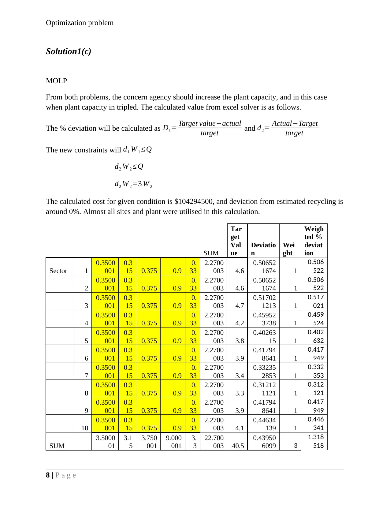
Solution1(c)
MOLP
From both problems, the concern agency should increase the plant capacity, and in this case
when plant capacity in tripled. The calculated value from excel solver is as follows.
The % deviation will be calculated as D1= Target value−actual
target and d2= Actual−Target
target
The new constraints will d1 W 1 ≤ Q
d2 W2 ≤ Q
d2 W2=3 W 2
The calculated cost for given condition is $104294500, and deviation from estimated recycling is
around 0%. Almost all sites and plant were utilised in this calculation.
SUM
Tar
get
Val
ue
Deviatio
n
Wei
ght
Weigh
ted %
deviat
ion
Sector 1
0.3500
001
0.3
15 0.375 0.9
0.
33
2.2700
003 4.6
0.50652
1674 1
0.506
522
2
0.3500
001
0.3
15 0.375 0.9
0.
33
2.2700
003 4.6
0.50652
1674 1
0.506
522
3
0.3500
001
0.3
15 0.375 0.9
0.
33
2.2700
003 4.7
0.51702
1213 1
0.517
021
4
0.3500
001
0.3
15 0.375 0.9
0.
33
2.2700
003 4.2
0.45952
3738 1
0.459
524
5
0.3500
001
0.3
15 0.375 0.9
0.
33
2.2700
003 3.8
0.40263
15 1
0.402
632
6
0.3500
001
0.3
15 0.375 0.9
0.
33
2.2700
003 3.9
0.41794
8641 1
0.417
949
7
0.3500
001
0.3
15 0.375 0.9
0.
33
2.2700
003 3.4
0.33235
2853 1
0.332
353
8
0.3500
001
0.3
15 0.375 0.9
0.
33
2.2700
003 3.3
0.31212
1121 1
0.312
121
9
0.3500
001
0.3
15 0.375 0.9
0.
33
2.2700
003 3.9
0.41794
8641 1
0.417
949
10
0.3500
001
0.3
15 0.375 0.9
0.
33
2.2700
003 4.1
0.44634
139 1
0.446
341
SUM
3.5000
01
3.1
5
3.750
001
9.000
001
3.
3
22.700
003 40.5
0.43950
6099 3
1.318
518
8 | P a g e
Optimization problem
The current scenario of MOLP result concludes that, the combined effect of MOLP is not
changing from individual effect of running solver for Cost and tonnage. In this condition it can
be suggested that, we must increase the recycling capacity by three times. If we increase the
efficiency then we can fulfil the requirement without increasing he capacity.
Solution 2
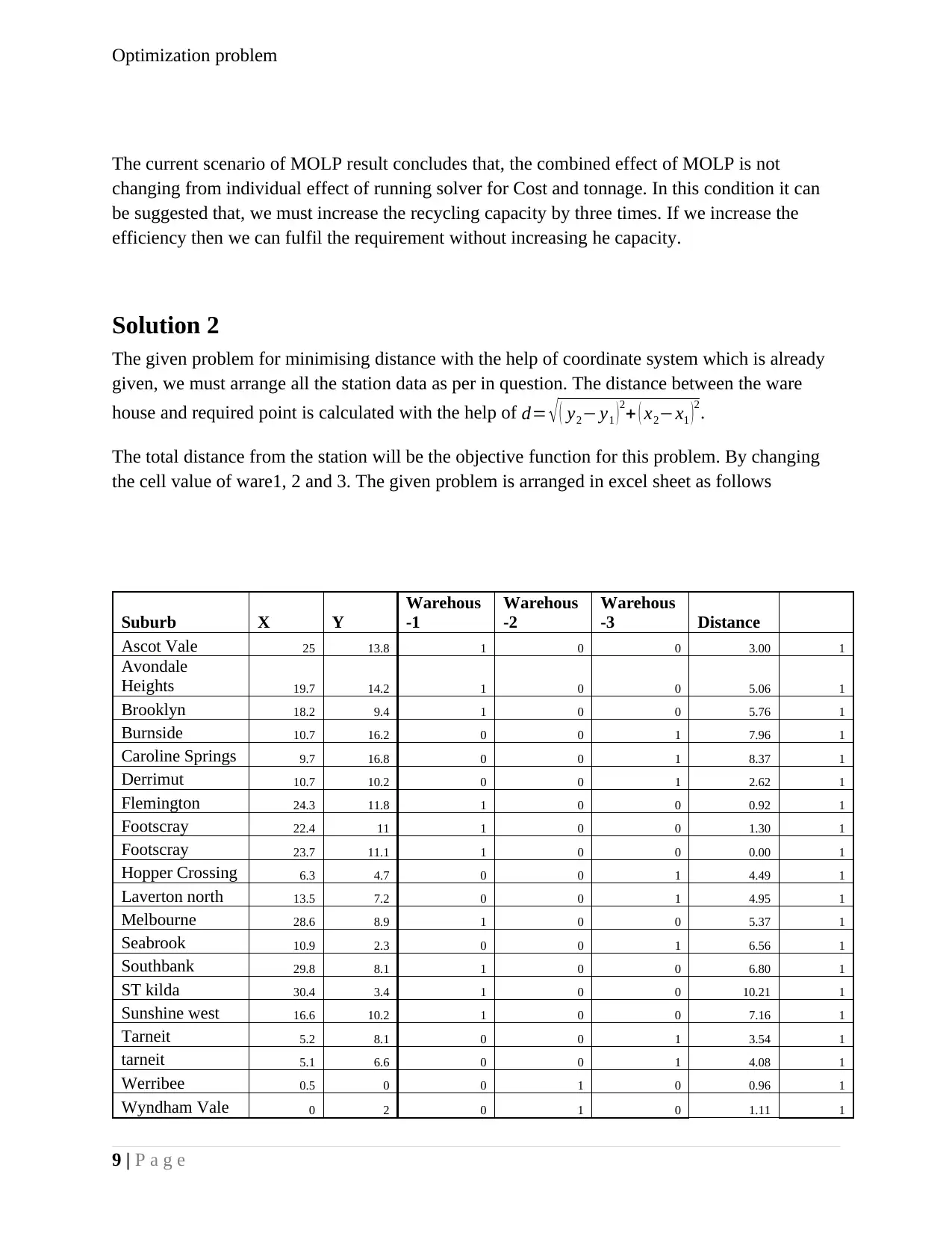
The given problem for minimising distance with the help of coordinate system which is already
given, we must arrange all the station data as per in question. The distance between the ware
house and required point is calculated with the help of d= √ ( y2− y1 ) 2+ ( x2−x1 ) 2.
The total distance from the station will be the objective function for this problem. By changing
the cell value of ware1, 2 and 3. The given problem is arranged in excel sheet as follows
Suburb X Y
Warehous
-1
Warehous
-2
Warehous
-3 Distance
Ascot Vale 25 13.8 1 0 0 3.00 1
Avondale
Heights 19.7 14.2 1 0 0 5.06 1
Brooklyn 18.2 9.4 1 0 0 5.76 1
Burnside 10.7 16.2 0 0 1 7.96 1
Caroline Springs 9.7 16.8 0 0 1 8.37 1
Derrimut 10.7 10.2 0 0 1 2.62 1
Flemington 24.3 11.8 1 0 0 0.92 1
Footscray 22.4 11 1 0 0 1.30 1
Footscray 23.7 11.1 1 0 0 0.00 1
Hopper Crossing 6.3 4.7 0 0 1 4.49 1
Laverton north 13.5 7.2 0 0 1 4.95 1
Melbourne 28.6 8.9 1 0 0 5.37 1
Seabrook 10.9 2.3 0 0 1 6.56 1
Southbank 29.8 8.1 1 0 0 6.80 1
ST kilda 30.4 3.4 1 0 0 10.21 1
Sunshine west 16.6 10.2 1 0 0 7.16 1
Tarneit 5.2 8.1 0 0 1 3.54 1
tarneit 5.1 6.6 0 0 1 4.08 1
Werribee 0.5 0 0 1 0 0.96 1
Wyndham Vale 0 2 0 1 0 1.11 1
9 | P a g e
The current scenario of MOLP result concludes that, the combined effect of MOLP is not
changing from individual effect of running solver for Cost and tonnage. In this condition it can
be suggested that, we must increase the recycling capacity by three times. If we increase the
efficiency then we can fulfil the requirement without increasing he capacity.
Solution 2
The given problem for minimising distance with the help of coordinate system which is already
given, we must arrange all the station data as per in question. The distance between the ware
house and required point is calculated with the help of d= √ ( y2− y1 ) 2+ ( x2−x1 ) 2.
The total distance from the station will be the objective function for this problem. By changing
the cell value of ware1, 2 and 3. The given problem is arranged in excel sheet as follows
Suburb X Y
Warehous
-1
Warehous
-2
Warehous
-3 Distance
Ascot Vale 25 13.8 1 0 0 3.00 1
Avondale
Heights 19.7 14.2 1 0 0 5.06 1
Brooklyn 18.2 9.4 1 0 0 5.76 1
Burnside 10.7 16.2 0 0 1 7.96 1
Caroline Springs 9.7 16.8 0 0 1 8.37 1
Derrimut 10.7 10.2 0 0 1 2.62 1
Flemington 24.3 11.8 1 0 0 0.92 1
Footscray 22.4 11 1 0 0 1.30 1
Footscray 23.7 11.1 1 0 0 0.00 1
Hopper Crossing 6.3 4.7 0 0 1 4.49 1
Laverton north 13.5 7.2 0 0 1 4.95 1
Melbourne 28.6 8.9 1 0 0 5.37 1
Seabrook 10.9 2.3 0 0 1 6.56 1
Southbank 29.8 8.1 1 0 0 6.80 1
ST kilda 30.4 3.4 1 0 0 10.21 1
Sunshine west 16.6 10.2 1 0 0 7.16 1
Tarneit 5.2 8.1 0 0 1 3.54 1
tarneit 5.1 6.6 0 0 1 4.08 1
Werribee 0.5 0 0 1 0 0.96 1
Wyndham Vale 0 2 0 1 0 1.11 1
9 | P a g e
⊘ This is a preview!⊘
Do you want full access?
Subscribe today to unlock all pages.
Trusted by 1+ million students worldwide
Optimization problem
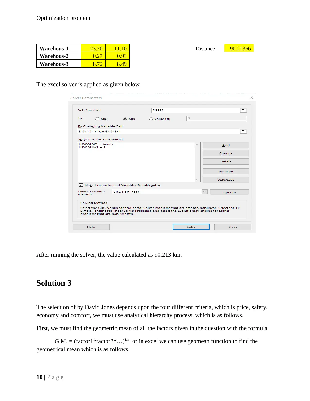
Warehous-1 23.70 11.10 Distance 90.21366
Warehous-2 0.27 0.93
Warehous-3 8.72 8.49
The excel solver is applied as given below
After running the solver, the value calculated as 90.213 km.
Solution 3
The selection of by David Jones depends upon the four different criteria, which is price, safety,
economy and comfort, we must use analytical hierarchy process, which is as follows.
First, we must find the geometric mean of all the factors given in the question with the formula
G.M. = (factor1*factor2*…)1/n, or in excel we can use geomean function to find the
geometrical mean which is as follows.
10 | P a g e
Paraphrase This Document
Need a fresh take? Get an instant paraphrase of this document with our AI Paraphraser
Optimization problem
Price Safety
Econom
y
Comfor
t G.M.
Price 1
0.16666
7
0.33333
3 0.2
0.32466791
5
Safety 6 1 4 2
2.63214802
6
Economy 3 0.25 1
0.33333
3
0.70710678
1
Comfort 5 0.5 3 1 1.65487546
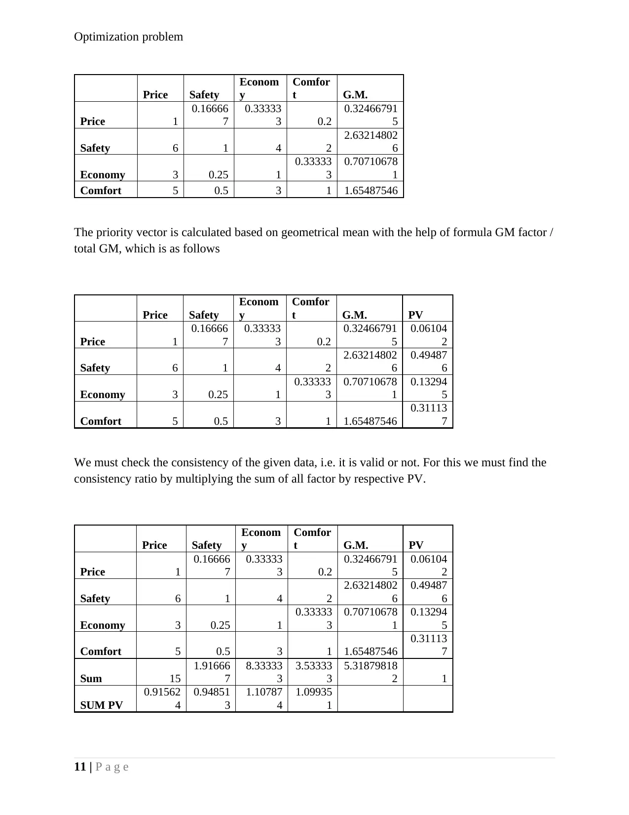
The priority vector is calculated based on geometrical mean with the help of formula GM factor /
total GM, which is as follows
Price Safety
Econom
y
Comfor
t G.M. PV
Price 1
0.16666
7
0.33333
3 0.2
0.32466791
5
0.06104
2
Safety 6 1 4 2
2.63214802
6
0.49487
6
Economy 3 0.25 1
0.33333
3
0.70710678
1
0.13294
5
Comfort 5 0.5 3 1 1.65487546
0.31113
7
We must check the consistency of the given data, i.e. it is valid or not. For this we must find the
consistency ratio by multiplying the sum of all factor by respective PV.
Price Safety
Econom
y
Comfor
t G.M. PV
Price 1
0.16666
7
0.33333
3 0.2
0.32466791
5
0.06104
2
Safety 6 1 4 2
2.63214802
6
0.49487
6
Economy 3 0.25 1
0.33333
3
0.70710678
1
0.13294
5
Comfort 5 0.5 3 1 1.65487546
0.31113
7
Sum 15
1.91666
7
8.33333
3
3.53333
3
5.31879818
2 1
SUM PV
0.91562
4
0.94851
3
1.10787
4
1.09935
1
11 | P a g e
Price Safety
Econom
y
Comfor
t G.M.
Price 1
0.16666
7
0.33333
3 0.2
0.32466791
5
Safety 6 1 4 2
2.63214802
6
Economy 3 0.25 1
0.33333
3
0.70710678
1
Comfort 5 0.5 3 1 1.65487546
The priority vector is calculated based on geometrical mean with the help of formula GM factor /
total GM, which is as follows
Price Safety
Econom
y
Comfor
t G.M. PV
Price 1
0.16666
7
0.33333
3 0.2
0.32466791
5
0.06104
2
Safety 6 1 4 2
2.63214802
6
0.49487
6
Economy 3 0.25 1
0.33333
3
0.70710678
1
0.13294
5
Comfort 5 0.5 3 1 1.65487546
0.31113
7
We must check the consistency of the given data, i.e. it is valid or not. For this we must find the
consistency ratio by multiplying the sum of all factor by respective PV.
Price Safety
Econom
y
Comfor
t G.M. PV
Price 1
0.16666
7
0.33333
3 0.2
0.32466791
5
0.06104
2
Safety 6 1 4 2
2.63214802
6
0.49487
6
Economy 3 0.25 1
0.33333
3
0.70710678
1
0.13294
5
Comfort 5 0.5 3 1 1.65487546
0.31113
7
Sum 15
1.91666
7
8.33333
3
3.53333
3
5.31879818
2 1
SUM PV
0.91562
4
0.94851
3
1.10787
4
1.09935
1
11 | P a g e
Optimization problem
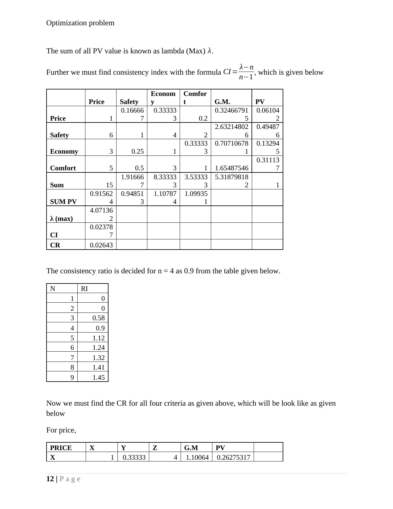
The sum of all PV value is known as lambda (Max) λ.
Further we must find consistency index with the formula CI = λ−n
n−1 , which is given below
Price Safety
Econom
y
Comfor
t G.M. PV
Price 1
0.16666
7
0.33333
3 0.2
0.32466791
5
0.06104
2
Safety 6 1 4 2
2.63214802
6
0.49487
6
Economy 3 0.25 1
0.33333
3
0.70710678
1
0.13294
5
Comfort 5 0.5 3 1 1.65487546
0.31113
7
Sum 15
1.91666
7
8.33333
3
3.53333
3
5.31879818
2 1
SUM PV
0.91562
4
0.94851
3
1.10787
4
1.09935
1
λ (max)
4.07136
2
CI
0.02378
7
CR 0.02643
The consistency ratio is decided for n = 4 as 0.9 from the table given below.
N RI
1 0
2 0
3 0.58
4 0.9
5 1.12
6 1.24
7 1.32
8 1.41
9 1.45
Now we must find the CR for all four criteria as given above, which will be look like as given
below
For price,
PRICE X Y Z G.M PV
X 1 0.33333 4 1.10064 0.26275317
12 | P a g e
⊘ This is a preview!⊘
Do you want full access?
Subscribe today to unlock all pages.
Trusted by 1+ million students worldwide
1 out of 19
Related Documents


Your All-in-One AI-Powered Toolkit for Academic Success.
+13062052269
info@desklib.com
Available 24*7 on WhatsApp / Email
![[object Object]](/_next/static/media/star-bottom.7253800d.svg)
Unlock your academic potential
Copyright © 2020–2026 A2Z Services. All Rights Reserved. Developed and managed by ZUCOL.