Long-Run Purchasing Power Parity Test Report Analysis 2017
VerifiedAdded on 2020/03/13
|34
|6385
|168
Report
AI Summary
This report investigates the long-run Purchasing Power Parity (PPP) theory, a fundamental concept in international economics, by examining data from the European region, United Kingdom, and the United States from 1988 to 2010. It explores the relationship between exchange rates and price levels, utilizing co-integration techniques and unit root tests, including Augmented Dickey-Fuller and Philips-Perron tests, to assess the stationarity of real exchange rates. The study aims to validate the PPP hypothesis, which suggests that exchange rates adjust to equalize the purchasing power of different currencies. The methodology involves regression analysis, unit root tests, and co-integration methods to determine if the real exchange rate remains constant over time. The findings are discussed in relation to previous research, including the work of Huan and Yang, and the implications for understanding the competitiveness of countries and their trading partners. The report concludes with a summary of the results, limitations, and suggestions for future research, contributing to the ongoing debate on the validity of PPP in the long run. This report also reviews literature to provide context for the analysis.
Test for Long-run Purchasing Power Parity (PPP)
Name
University
22nd August 2017
Name
University
22nd August 2017
Paraphrase This Document
Need a fresh take? Get an instant paraphrase of this document with our AI Paraphraser
INTRODUCTION
Purchasing power parity (PPP) is a balance condition that is frequently accepted in both
hypothetical and useful monetary examination. Observational testing of PPP has not, however,
gave clear proof that legitimizes its expansive application - despite what might be expected,
various examinations have achieved negative conclusions with respect to its validity. This paper
endeavors to accommodate the wide utilization of purchasing power equality and the
experimental confirmation, by utilizing more proper techniques to test the speculation, inside a
multivariate and multi-nation setting for European region, United Kingdom, and the United
States in the period 1988-2010.
In its supreme rendition, the theory of purchasing power parity builds up that the value levels of
two nations ought to be equivalent when expressed in a similar currency. In this manner,
P=SP∗¿
Where S is the nominal exchange rate of the currency of country A expressed in terms of the
currency of country B, and P and P* the price levels of countries A and B, respectively. This
version of PPP implies, therefore, that the logarithm of the real exchange rate is constant and
equal to zero.
The theory of long-run purchasing power parity (PPP) states that monetary standards of various
nations have a similar buying power within the sight of universal arbitrage. Testing the
hypothesis for the long-run PPP gives a valuable understanding into whether the country's
competitiveness and its trading partners, based on the real exchange rate, fluctuates or remains
steady after some time. Previous studies heavily depended upon standard econometric techniques
when it came to testing the long-run PPP. The disappointment experienced from these
procedures especially to consider the economic time series non-stationary behavior brings about
what has turned out to be known as "spurious regressions."
Modeling techniques such as co-integration have been able to detect the presence of long-run
equilibrium associations that exist between non-stationary variables, with this, the long-run PPP
theory has therefore been getting restored consideration.
Notwithstanding whether the theory of long-run PPP remains constant or not, the examiner's
decision of the co-integration approach, regardless of whether it is the Granger and Engle two
stage strategy or the Juselius and Johansen multivariate procedure, ought not have any
noteworthy effect upon the result of the hypothesis test. Notwithstanding, in one of the recent
studies, Huan and Yang (1996) concluded that when the Granger and Engle technique rejects the
long-run PPP theory the Juseliusand Johansen technique has a tendency to acknowledge
it.Through Monte Carlo simulations utilizing data from France, Canada, Switzerland, Germany,
the U.S.A., and the U.K., Huan and Yang found that the Juselius and Johansen co-integration
strategy is one-sided toward supporting the long-run PPP under conditions in which the
presumption of ordinarily as well as autonomously and indistinguishably appropriated
aggravation term is violated.
This paper applies the two co-integration strategies to consumer price index (CPI) and exchange
rate data from three developed regions to test for the long-run PPP speculation. In particular, it
tests whether Huan and Yang's claim, that the two co-integration systems yield contradicting
outcomes, remains constant with regards to developed regions. The two co-integration
approaches are applied to a time series data spanning from 1988 to 2010. The paper utilizes
effective exchange rate as the measure of exchange rate. Most countries have more than one
exchanging partner, the effective exchange rate is the suitable measure of exchange rate (Officer
(1980)).
The early experimental has grounded for a long time to look at the purchasing power parity
(PPP) exchange rates proved by statistical estimations and discovering versatility coefficients on
residential and foreign costs. Frankel (1978) conducted a study on relative and absolute PPP
convention amid the adaptable exchange rates. His outcome discovered causality relationship of
exchange rate on cost in the sense of granger. Most traditional econometric estimations such as
least square approach (GLS) in view of non-stationary time series results to spurious regression
and statistics may essentially show only correlated trends as opposed to a genuine relationship
(Granger and Newbold, 1974). Augmented Dickey-Fuller (1981) and Philips and Perron, (1988)
tests can help maintain a strategic distance from false outcomes through stationary tests of times
series.
Based on this, a number of observational studies present progression in the estimated equation of
PPP. Abuaf and Jorian (1990), conducted a unit-root test for non-stationary time series data.
Their results do not bolster PPP in long-run of the significant monetary forms. Taylor (1988)
utilized a co-integration of Johansen approach (1988) to conclude that there is a no connection
amongst costs and exchange rate. Patel (1990) utilized Engel-granger co-integration strategy to
affirm purchasing power parity prove. They pointed in their outcomes unfavorable proof to PPP
hypothesis amid the 1971-period assessed as ridiculing period after the Nixon (1993) inspected
long-run purchasing power parity utilizing a partial co-integration examination for the period
1914 - 1989. Their results upheld PPP as a long-run approach.
Johnson (1990) identified a solid and long-run U.S. - Canada data PPP idea. Philip (2001)
affirmed the confirmation of PPP in small-sample from yearly data spreading over 1973 through
1997 Nominal exchange rates for France, Canada, Japan, Italy, U.K and Switzerland are relative
to the U.S. dollar. Rogoff (1996)found out that PPP hypothesis did not hold amongst developing
and developed countries. Haug and Besher (2007) established a sort of mixed outcomes for non–
linear and linear co-integration in the PPP model utilizing monthly data from the post-Bretton
Woods period for G-10 nations. Ozdemir (2008), established bolster for PPP either over the long
⊘ This is a preview!⊘
Do you want full access?
Subscribe today to unlock all pages.
Trusted by 1+ million students worldwide
run. Hyrina and Serletis (2010) looked at various econometric strategies utilized in earlier and
later studies to verify PPP idea, where early experimental techniques failed to recognize PPP
presence contrasted with current investigations.
Hussein (2015) analyzed the long run development between US dollar and Canadian dollar
exchange rates upon month to month data for the period 1995 to 2008 utilizing the Engle-
Granger co-integration test. In his paper, he doesn't give the validity of PPP between US dollar
and Canadian dollar trade rates. Pedroni (2001) showed blended proof of PPP in view of panel
unit root tests. He showed the presence of weak PPP and rejected solid PPP idea. Robertson et al
(2014) utilized panel co-integration approach of month to month data from 1982 through to 2010
to explore the Purchasing Power Parity (PPP) between the Mexico and US.
The rest of the paper is organized in the following way. The literature review on the theory of
long-run PPP is presented in section II. Section III introduces the methodology used which
includes the approaches, philosophies, strategies and justification of the approaches used. Section
IV presents the empirical findings based on the analysis of data. Section V provides discussion of
the findings and interpretation of the results. Lastly, section VI provides the conclusions,
limitations of the study and a brief summary of the entire paper.
METHODOLOGY
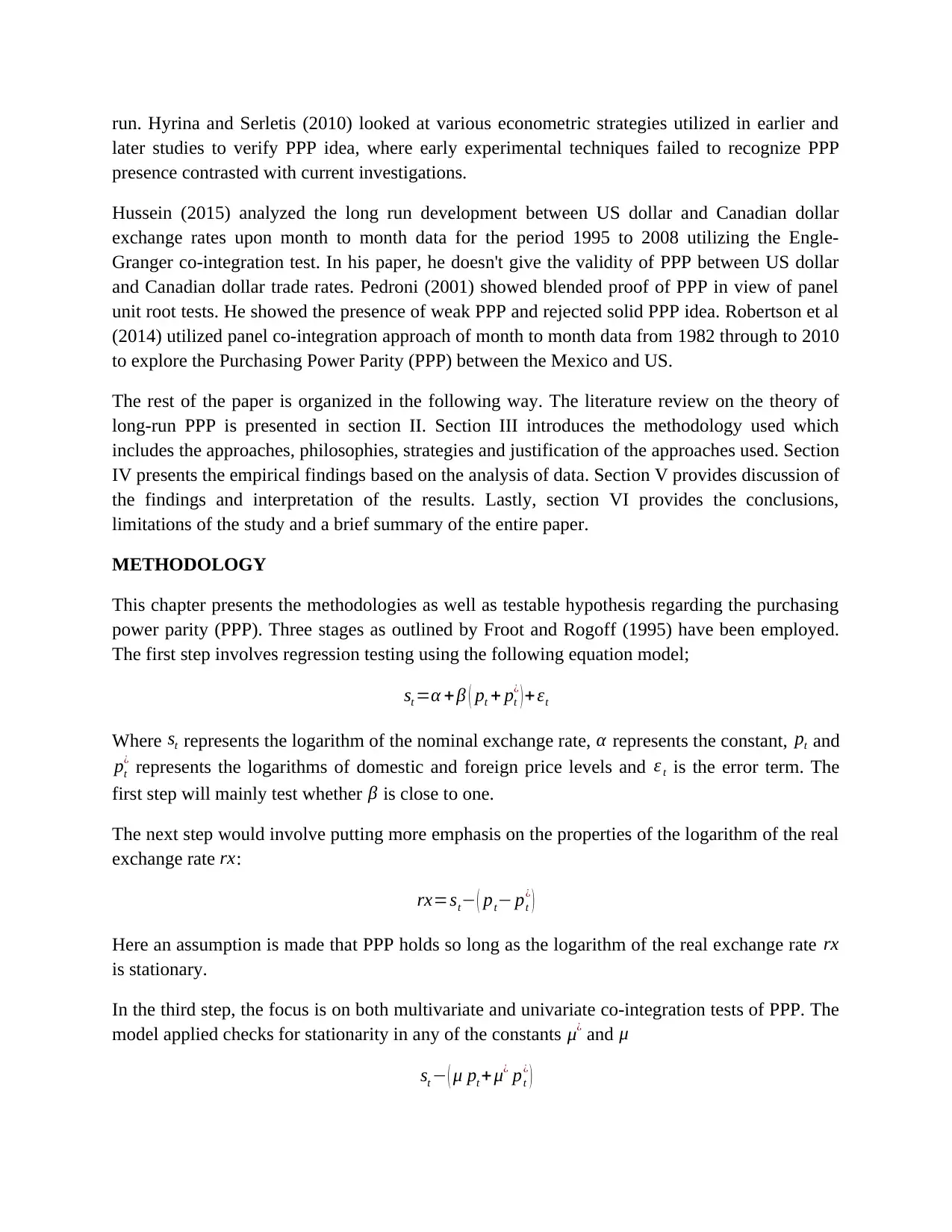
This chapter presents the methodologies as well as testable hypothesis regarding the purchasing
power parity (PPP). Three stages as outlined by Froot and Rogoff (1995) have been employed.
The first step involves regression testing using the following equation model;
st =α +β ( pt + pt
¿
) +εt
Where st represents the logarithm of the nominal exchange rate, α represents the constant, pt and
pt
¿ represents the logarithms of domestic and foreign price levels and ε t is the error term. The
first step will mainly test whether β is close to one.
The next step would involve putting more emphasis on the properties of the logarithm of the real
exchange rate rx:
rx=st− ( pt− pt
¿
)
Here an assumption is made that PPP holds so long as the logarithm of the real exchange rate rx
is stationary.
In the third step, the focus is on both multivariate and univariate co-integration tests of PPP. The
model applied checks for stationarity in any of the constants μ¿ and μ
st − ( μ pt + μ¿ pt
¿
)
later studies to verify PPP idea, where early experimental techniques failed to recognize PPP
presence contrasted with current investigations.
Hussein (2015) analyzed the long run development between US dollar and Canadian dollar
exchange rates upon month to month data for the period 1995 to 2008 utilizing the Engle-
Granger co-integration test. In his paper, he doesn't give the validity of PPP between US dollar
and Canadian dollar trade rates. Pedroni (2001) showed blended proof of PPP in view of panel
unit root tests. He showed the presence of weak PPP and rejected solid PPP idea. Robertson et al
(2014) utilized panel co-integration approach of month to month data from 1982 through to 2010
to explore the Purchasing Power Parity (PPP) between the Mexico and US.
The rest of the paper is organized in the following way. The literature review on the theory of
long-run PPP is presented in section II. Section III introduces the methodology used which
includes the approaches, philosophies, strategies and justification of the approaches used. Section
IV presents the empirical findings based on the analysis of data. Section V provides discussion of
the findings and interpretation of the results. Lastly, section VI provides the conclusions,
limitations of the study and a brief summary of the entire paper.
METHODOLOGY
This chapter presents the methodologies as well as testable hypothesis regarding the purchasing
power parity (PPP). Three stages as outlined by Froot and Rogoff (1995) have been employed.
The first step involves regression testing using the following equation model;
st =α +β ( pt + pt
¿
) +εt
Where st represents the logarithm of the nominal exchange rate, α represents the constant, pt and
pt
¿ represents the logarithms of domestic and foreign price levels and ε t is the error term. The
first step will mainly test whether β is close to one.
The next step would involve putting more emphasis on the properties of the logarithm of the real
exchange rate rx:
rx=st− ( pt− pt
¿
)
Here an assumption is made that PPP holds so long as the logarithm of the real exchange rate rx
is stationary.
In the third step, the focus is on both multivariate and univariate co-integration tests of PPP. The
model applied checks for stationarity in any of the constants μ¿ and μ
st − ( μ pt + μ¿ pt
¿
)
Paraphrase This Document
Need a fresh take? Get an instant paraphrase of this document with our AI Paraphraser
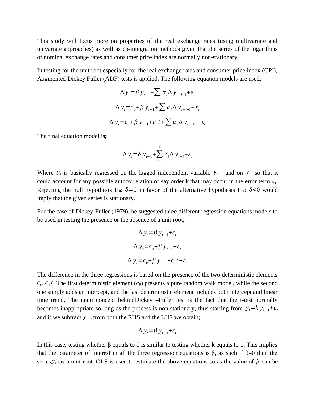
This study will focus more on properties of the real exchange rates (using multivariate and
univariate approaches) as well as co-integration methods given that the series of the logarithms
of nominal exchange rates and consumer price index are normally non-stationary.
In testing for the unit root especially for the real exchange rates and consumer price index (CPI),
Augmented Dickey Fuller (ADF) tests is applied. The following equation models are used;
∆ yt =β yt−1 +∑ αi ∆ yt−i+1 + εt
∆ yt =c0 + β yt−1 +∑ α i ∆ yt−i+1 + εt
∆ yt =c0 + β yt−1 +c1 t +∑ α i ∆ yt−i+1 + εt
The final equation model is;
∆ yt =δ yt−1 +∑
i=1
k
δi ∆ yt−i +εt
Where yt is basically regressed on the lagged independent variable yt −1 and on yt −iso that it
could account for any possible autocorrelation of say order k that may occur in the error term ε t.
Rejecting the null hypothesis H0: δ=0 in favor of the alternative hypothesis HA: δ <0 would
imply that the given series is stationary.
For the case of Dickey-Fuller (1979), he suggested three different regression equations models to
be used in testing the presence or the absence of a unit root;
∆ yt =β yt−1 +εt
∆ yt =c0 + β yt−1 +εt
∆ yt =c0 + β yt−1 +c1 t +εt
The difference in the three regressions is based on the presence of the two deterministic elements
c0, c1 t. The first deterministic element (c0) presents a pure random walk model, while the second
one simply adds an intercept, and the last deterministic element includes both intercept and linear
time trend. The main concept behindDickey –Fuller test is the fact that the t-test normally
becomes inappropriate so long as the process is non-stationary, thus starting from yt =k yt −1 +εt
and if we subtract yt −1from both the RHS and the LHS we obtain;
∆ yt =β yt−1 +εt
In this case, testing whether β equals to 0 is similar to testing whether k equals to 1. This implies
that the parameter of interest in all the three regression equations is β, as such if β=0 then the
series ythas a unit root. OLS is used to estimate the above equations so as the value of β can be
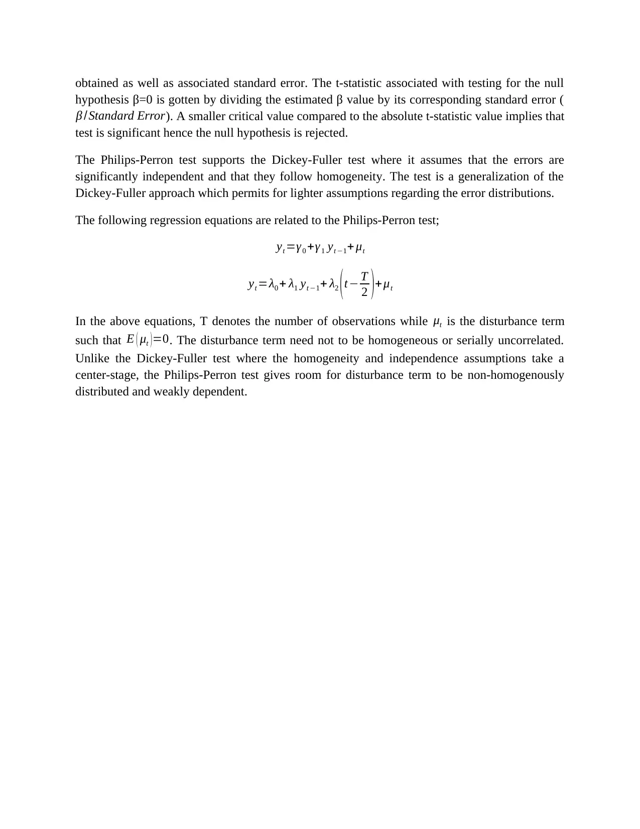
obtained as well as associated standard error. The t-statistic associated with testing for the null
hypothesis β=0 is gotten by dividing the estimated β value by its corresponding standard error (
β / Standard Error). A smaller critical value compared to the absolute t-statistic value implies that
test is significant hence the null hypothesis is rejected.
The Philips-Perron test supports the Dickey-Fuller test where it assumes that the errors are
significantly independent and that they follow homogeneity. The test is a generalization of the
Dickey-Fuller approach which permits for lighter assumptions regarding the error distributions.
The following regression equations are related to the Philips-Perron test;
yt =γ 0 +γ 1 yt −1+ μt
yt =λ0 + λ1 yt −1+ λ2 (t− T
2 )+μt
In the above equations, T denotes the number of observations while μt is the disturbance term
such that E ( μt )=0. The disturbance term need not to be homogeneous or serially uncorrelated.
Unlike the Dickey-Fuller test where the homogeneity and independence assumptions take a
center-stage, the Philips-Perron test gives room for disturbance term to be non-homogenously
distributed and weakly dependent.
⊘ This is a preview!⊘
Do you want full access?
Subscribe today to unlock all pages.
Trusted by 1+ million students worldwide
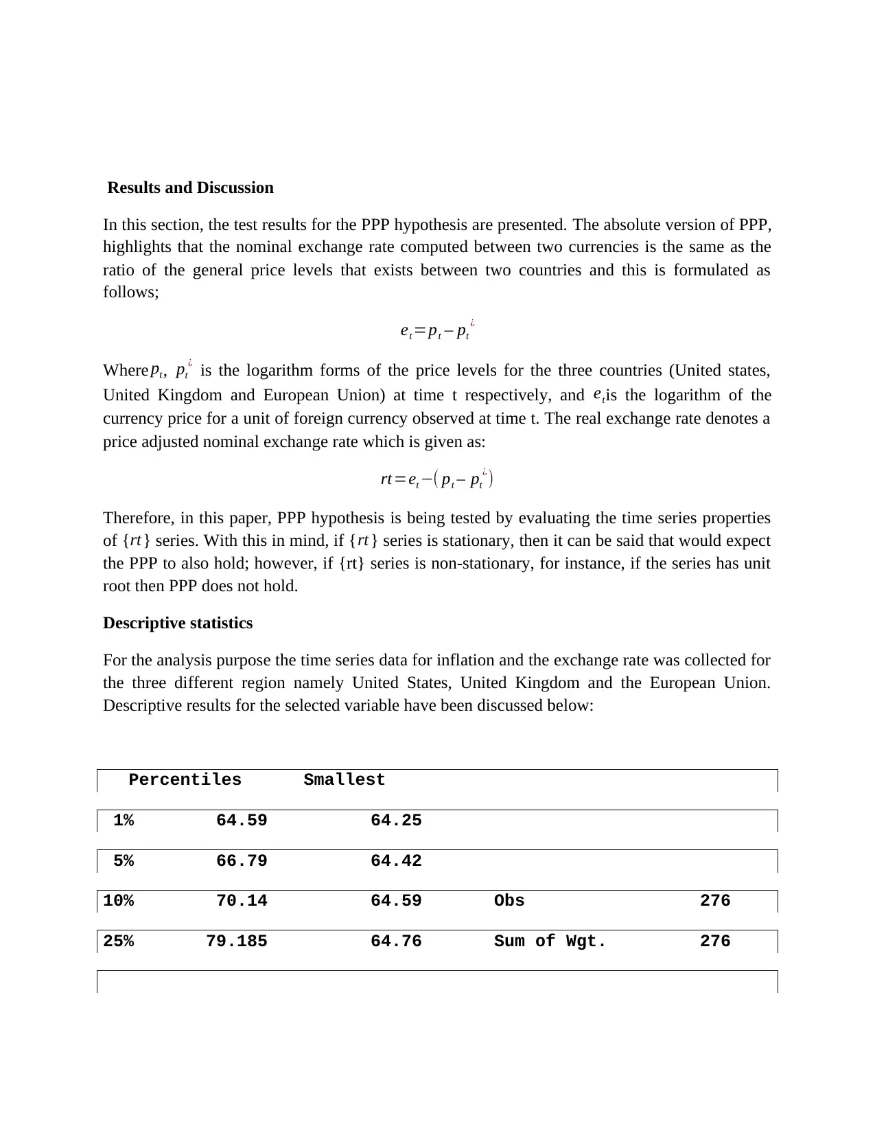
Results and Discussion
In this section, the test results for the PPP hypothesis are presented. The absolute version of PPP,
highlights that the nominal exchange rate computed between two currencies is the same as the
ratio of the general price levels that exists between two countries and this is formulated as
follows;
et =pt – pt
¿
Where pt, pt
¿ is the logarithm forms of the price levels for the three countries (United states,
United Kingdom and European Union) at time t respectively, and etis the logarithm of the
currency price for a unit of foreign currency observed at time t. The real exchange rate denotes a
price adjusted nominal exchange rate which is given as:
rt=et −( pt – pt
¿)
Therefore, in this paper, PPP hypothesis is being tested by evaluating the time series properties
of {rt} series. With this in mind, if { rt} series is stationary, then it can be said that would expect
the PPP to also hold; however, if {rt} series is non-stationary, for instance, if the series has unit
root then PPP does not hold.
Descriptive statistics
For the analysis purpose the time series data for inflation and the exchange rate was collected for
the three different region namely United States, United Kingdom and the European Union.
Descriptive results for the selected variable have been discussed below:
Percentiles Smallest
1% 64.59 64.25
5% 66.79 64.42
10% 70.14 64.59 Obs 276
25% 79.185 64.76 Sum of Wgt. 276
Paraphrase This Document
Need a fresh take? Get an instant paraphrase of this document with our AI Paraphraser
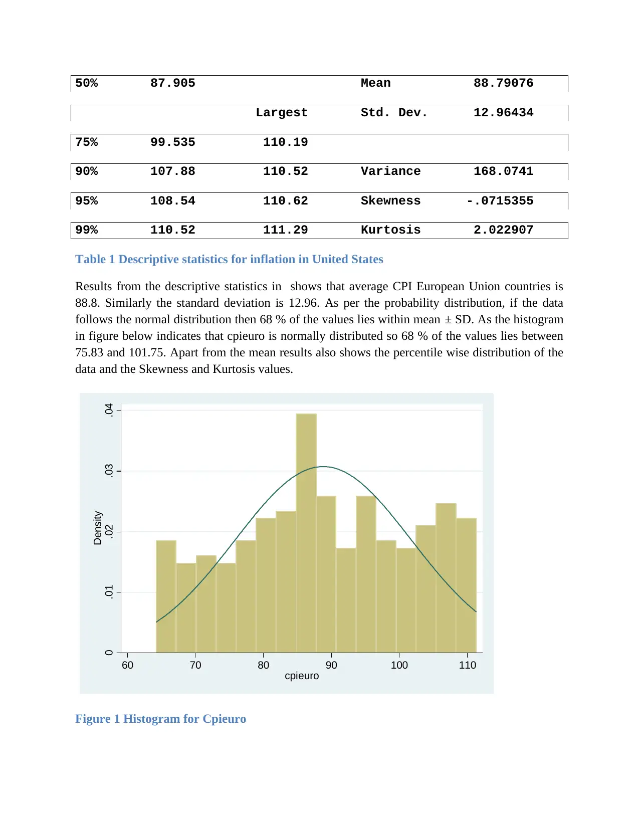
50% 87.905 Mean 88.79076
Largest Std. Dev. 12.96434
75% 99.535 110.19
90% 107.88 110.52 Variance 168.0741
95% 108.54 110.62 Skewness -.0715355
99% 110.52 111.29 Kurtosis 2.022907
Table 1 Descriptive statistics for inflation in United States
Results from the descriptive statistics in shows that average CPI European Union countries is
88.8. Similarly the standard deviation is 12.96. As per the probability distribution, if the data
follows the normal distribution then 68 % of the values lies within mean ± SD. As the histogram
in figure below indicates that cpieuro is normally distributed so 68 % of the values lies between
75.83 and 101.75. Apart from the mean results also shows the percentile wise distribution of the
data and the Skewness and Kurtosis values.
0 .01 .02 .03 .04
Density
60 70 80 90 100 110
cpieuro
Figure 1 Histogram for Cpieuro
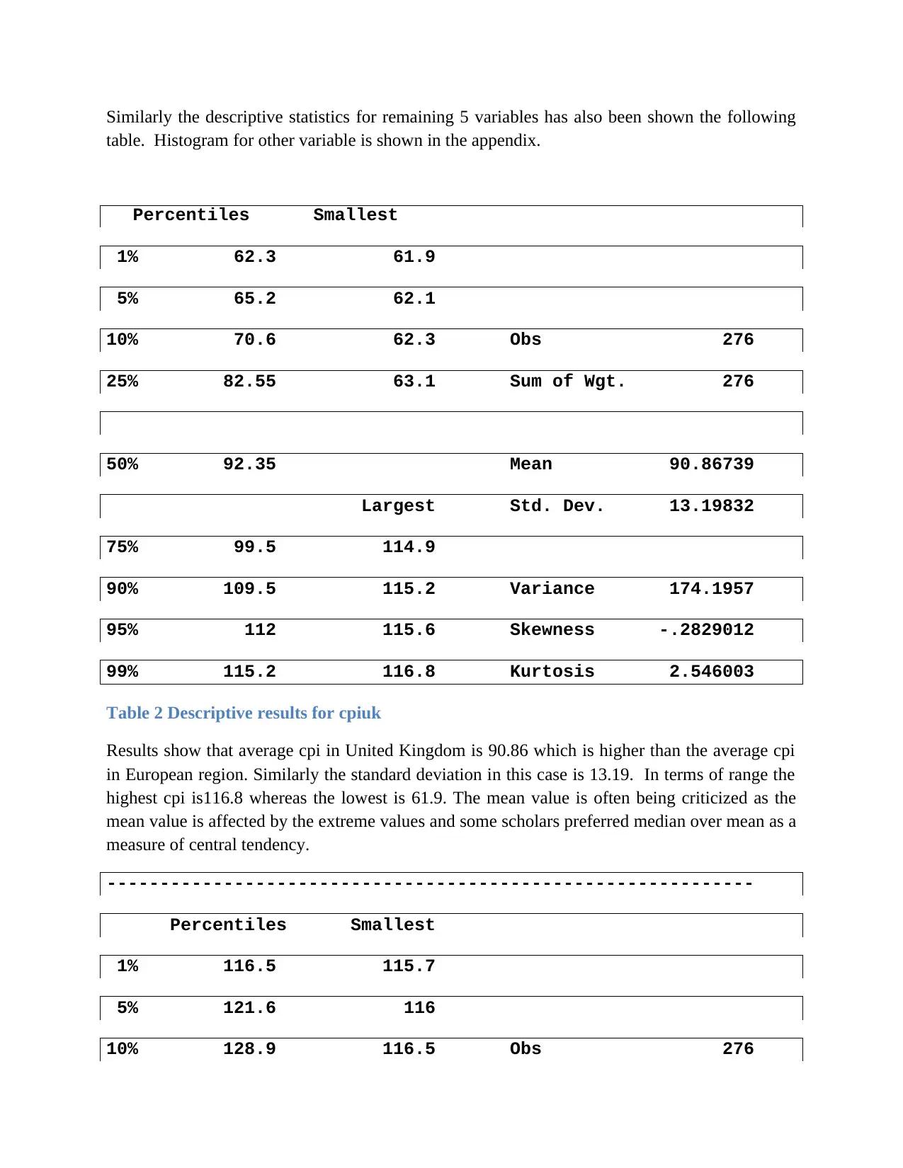
Similarly the descriptive statistics for remaining 5 variables has also been shown the following
table. Histogram for other variable is shown in the appendix.
Percentiles Smallest
1% 62.3 61.9
5% 65.2 62.1
10% 70.6 62.3 Obs 276
25% 82.55 63.1 Sum of Wgt. 276
50% 92.35 Mean 90.86739
Largest Std. Dev. 13.19832
75% 99.5 114.9
90% 109.5 115.2 Variance 174.1957
95% 112 115.6 Skewness -.2829012
99% 115.2 116.8 Kurtosis 2.546003
Table 2 Descriptive results for cpiuk
Results show that average cpi in United Kingdom is 90.86 which is higher than the average cpi
in European region. Similarly the standard deviation in this case is 13.19. In terms of range the
highest cpi is116.8 whereas the lowest is 61.9. The mean value is often being criticized as the
mean value is affected by the extreme values and some scholars preferred median over mean as a
measure of central tendency.
-------------------------------------------------------------
Percentiles Smallest
1% 116.5 115.7
5% 121.6 116
10% 128.9 116.5 Obs 276
⊘ This is a preview!⊘
Do you want full access?
Subscribe today to unlock all pages.
Trusted by 1+ million students worldwide
25% 145.4 117.1 Sum of Wgt. 276
50% 166.45 Mean 169.3701
Largest Std. Dev. 29.73352
75% 193.85 218.815
90% 213.528 219.086 Variance 884.0823
95% 217.631 219.179 Skewness .0749122
99% 219.086 219.964 Kurtosis 1.928545
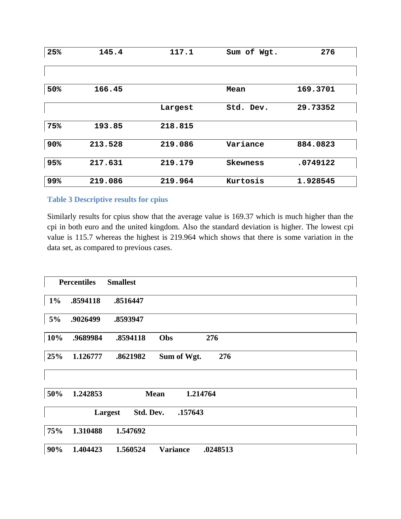
Table 3 Descriptive results for cpius
Similarly results for cpius show that the average value is 169.37 which is much higher than the
cpi in both euro and the united kingdom. Also the standard deviation is higher. The lowest cpi
value is 115.7 whereas the highest is 219.964 which shows that there is some variation in the
data set, as compared to previous cases.
Percentiles Smallest
1% .8594118 .8516447
5% .9026499 .8593947
10% .9689984 .8594118 Obs 276
25% 1.126777 .8621982 Sum of Wgt. 276
50% 1.242853 Mean 1.214764
Largest Std. Dev. .157643
75% 1.310488 1.547692
90% 1.404423 1.560524 Variance .0248513
50% 166.45 Mean 169.3701
Largest Std. Dev. 29.73352
75% 193.85 218.815
90% 213.528 219.086 Variance 884.0823
95% 217.631 219.179 Skewness .0749122
99% 219.086 219.964 Kurtosis 1.928545
Table 3 Descriptive results for cpius
Similarly results for cpius show that the average value is 169.37 which is much higher than the
cpi in both euro and the united kingdom. Also the standard deviation is higher. The lowest cpi
value is 115.7 whereas the highest is 219.964 which shows that there is some variation in the
data set, as compared to previous cases.
Percentiles Smallest
1% .8594118 .8516447
5% .9026499 .8593947
10% .9689984 .8594118 Obs 276
25% 1.126777 .8621982 Sum of Wgt. 276
50% 1.242853 Mean 1.214764
Largest Std. Dev. .157643
75% 1.310488 1.547692
90% 1.404423 1.560524 Variance .0248513
Paraphrase This Document
Need a fresh take? Get an instant paraphrase of this document with our AI Paraphraser
95% 1.461457 1.580327 Skewness -.3843775
99% 1.560524 1.597132 Kurtosis 2.853423
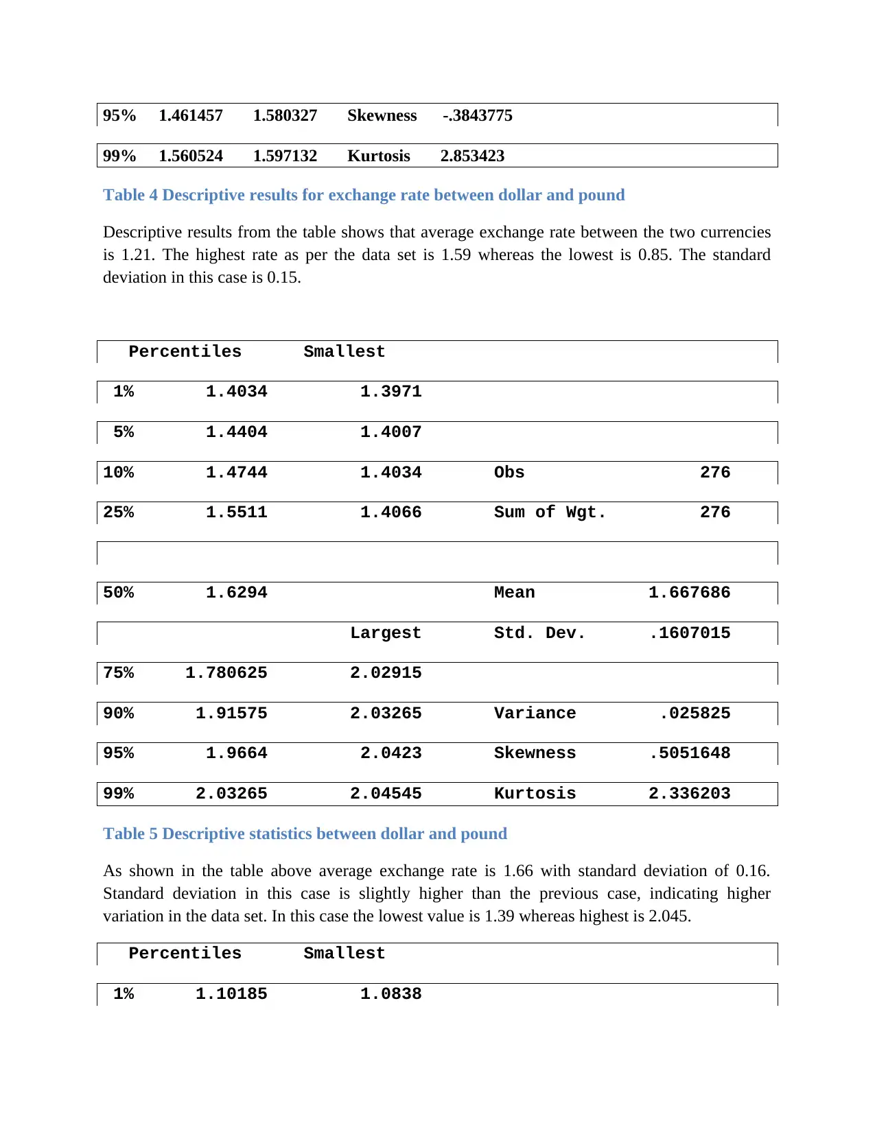
Table 4 Descriptive results for exchange rate between dollar and pound
Descriptive results from the table shows that average exchange rate between the two currencies
is 1.21. The highest rate as per the data set is 1.59 whereas the lowest is 0.85. The standard
deviation in this case is 0.15.
Percentiles Smallest
1% 1.4034 1.3971
5% 1.4404 1.4007
10% 1.4744 1.4034 Obs 276
25% 1.5511 1.4066 Sum of Wgt. 276
50% 1.6294 Mean 1.667686
Largest Std. Dev. .1607015
75% 1.780625 2.02915
90% 1.91575 2.03265 Variance .025825
95% 1.9664 2.0423 Skewness .5051648
99% 2.03265 2.04545 Kurtosis 2.336203
Table 5 Descriptive statistics between dollar and pound
As shown in the table above average exchange rate is 1.66 with standard deviation of 0.16.
Standard deviation in this case is slightly higher than the previous case, indicating higher
variation in the data set. In this case the lowest value is 1.39 whereas highest is 2.045.
Percentiles Smallest
1% 1.10185 1.0838
99% 1.560524 1.597132 Kurtosis 2.853423
Table 4 Descriptive results for exchange rate between dollar and pound
Descriptive results from the table shows that average exchange rate between the two currencies
is 1.21. The highest rate as per the data set is 1.59 whereas the lowest is 0.85. The standard
deviation in this case is 0.15.
Percentiles Smallest
1% 1.4034 1.3971
5% 1.4404 1.4007
10% 1.4744 1.4034 Obs 276
25% 1.5511 1.4066 Sum of Wgt. 276
50% 1.6294 Mean 1.667686
Largest Std. Dev. .1607015
75% 1.780625 2.02915
90% 1.91575 2.03265 Variance .025825
95% 1.9664 2.0423 Skewness .5051648
99% 2.03265 2.04545 Kurtosis 2.336203
Table 5 Descriptive statistics between dollar and pound
As shown in the table above average exchange rate is 1.66 with standard deviation of 0.16.
Standard deviation in this case is slightly higher than the previous case, indicating higher
variation in the data set. In this case the lowest value is 1.39 whereas highest is 2.045.
Percentiles Smallest
1% 1.10185 1.0838
5% 1.1428 1.08875
10% 1.18136 1.10185 Obs 276
25% 1.263585 1.11495 Sum of Wgt. 276
50% 1.417225 Mean 1.386635
Largest Std. Dev. .1458609
75% 1.48465 1.6529
90% 1.5929 1.6602 Variance .0212754
95% 1.6225 1.6621 Skewness -.114234
99% 1.6602 1.7 Kurtosis 2.095064
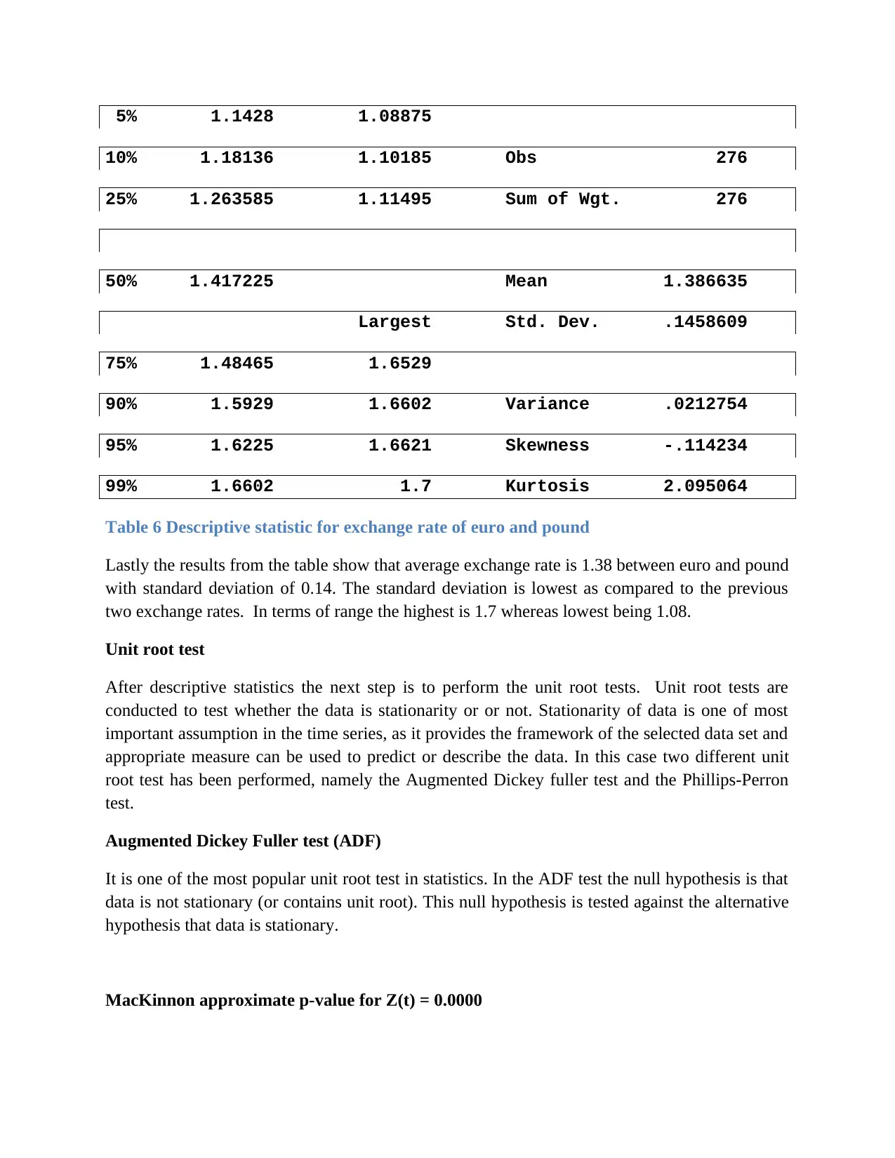
Table 6 Descriptive statistic for exchange rate of euro and pound
Lastly the results from the table show that average exchange rate is 1.38 between euro and pound
with standard deviation of 0.14. The standard deviation is lowest as compared to the previous
two exchange rates. In terms of range the highest is 1.7 whereas lowest being 1.08.
Unit root test
After descriptive statistics the next step is to perform the unit root tests. Unit root tests are
conducted to test whether the data is stationarity or or not. Stationarity of data is one of most
important assumption in the time series, as it provides the framework of the selected data set and
appropriate measure can be used to predict or describe the data. In this case two different unit
root test has been performed, namely the Augmented Dickey fuller test and the Phillips-Perron
test.
Augmented Dickey Fuller test (ADF)
It is one of the most popular unit root test in statistics. In the ADF test the null hypothesis is that
data is not stationary (or contains unit root). This null hypothesis is tested against the alternative
hypothesis that data is stationary.
MacKinnon approximate p-value for Z(t) = 0.0000
10% 1.18136 1.10185 Obs 276
25% 1.263585 1.11495 Sum of Wgt. 276
50% 1.417225 Mean 1.386635
Largest Std. Dev. .1458609
75% 1.48465 1.6529
90% 1.5929 1.6602 Variance .0212754
95% 1.6225 1.6621 Skewness -.114234
99% 1.6602 1.7 Kurtosis 2.095064
Table 6 Descriptive statistic for exchange rate of euro and pound
Lastly the results from the table show that average exchange rate is 1.38 between euro and pound
with standard deviation of 0.14. The standard deviation is lowest as compared to the previous
two exchange rates. In terms of range the highest is 1.7 whereas lowest being 1.08.
Unit root test
After descriptive statistics the next step is to perform the unit root tests. Unit root tests are
conducted to test whether the data is stationarity or or not. Stationarity of data is one of most
important assumption in the time series, as it provides the framework of the selected data set and
appropriate measure can be used to predict or describe the data. In this case two different unit
root test has been performed, namely the Augmented Dickey fuller test and the Phillips-Perron
test.
Augmented Dickey Fuller test (ADF)
It is one of the most popular unit root test in statistics. In the ADF test the null hypothesis is that
data is not stationary (or contains unit root). This null hypothesis is tested against the alternative
hypothesis that data is stationary.
MacKinnon approximate p-value for Z(t) = 0.0000
⊘ This is a preview!⊘
Do you want full access?
Subscribe today to unlock all pages.
Trusted by 1+ million students worldwide
1 out of 34
Your All-in-One AI-Powered Toolkit for Academic Success.
+13062052269
info@desklib.com
Available 24*7 on WhatsApp / Email
![[object Object]](/_next/static/media/star-bottom.7253800d.svg)
Unlock your academic potential
Copyright © 2020–2026 A2Z Services. All Rights Reserved. Developed and managed by ZUCOL.