MA5509 Numerical Methods: Error Analysis and Root-Finding Methods

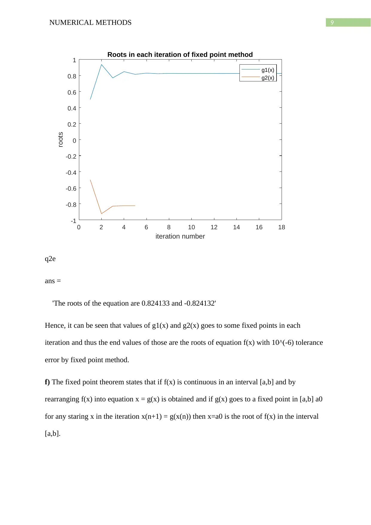
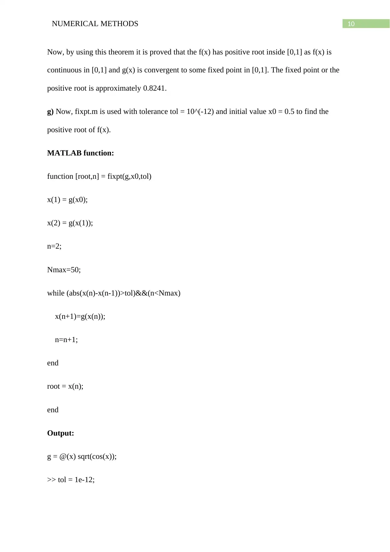
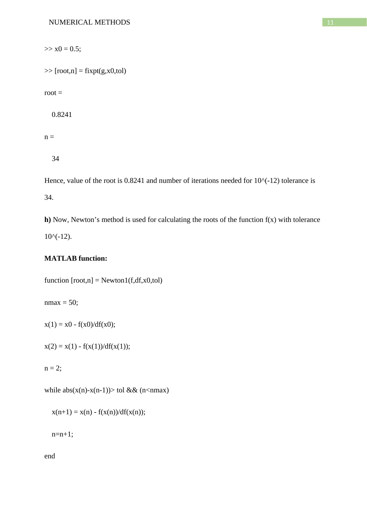
This document presents a solution to a Numerical Methods assignment, focusing on error analysis and root-finding techniques. The solution begins by determining the intervals for a given number to approximate x with a specified relative error, using MATLAB for calculations and visualizations. The assignment further explores the function f(x) = x^2 – cos(x), proving the existence and uniqueness of roots within specified intervals. The bisection algorithm is applied to approximate the positive root, with iterations and tolerance levels defined. The fixed-point iteration method is then implemented using MATLAB to calculate roots, followed by an explanation of the fixed-point theorem. Finally, Newton's method is utilized to calculate the roots with a defined tolerance. The assignment uses MATLAB functions and provides detailed explanations of each step, offering a comprehensive approach to solving numerical problems. Desklib provides a platform to explore similar assignments and past papers.

Running head: NUMERICAL METHODS
NUMERICAL METHODS
Name of the Student
Name of the University
Author Note

1NUMERICAL METHODS
1. a) Given, x = 10^3.
Now, the interval I inside which any number that approximates x will have a relative error <=
10^(-4) is calculated as follows.
Relative error = Absolute error/actual number
 Absolute error = Relative error*actual number
 Absolute error = Relative error*10^3.
Now, in MATLAB the relative error for different numbers is taken within the range 0 to
10^(-4) and the Absolute errors are calculated for the corresponding relative errors.
Theoretically, the max absolute error is calculated as follows.
Max Absolute error = Max Relative error * 10^(3) = 10^(-4) *10^(3) = 0.1.
MATLAB function:
r_err = linspace(0,1e-4,100);
x = 1e3;
abs_err = r_err.*x;
plot(r_err,abs_err,'r-')
title('relative error vs absolute error')
xlabel('relative error')
ylabel('absolute error')
Output:

2NUMERICAL METHODS
0 0.2 0.4 0.6 0.8 1 1.2
relative error 10-4
0
0.01
0.02
0.03
0.04
0.05
0.06
0.07
0.08
0.09
0.1
absolute error
relative error vs absolute error
maxabs =
0.1000
Now, the maximum absolute error is 0.1.
b) Now, when x = 10^(-2) then the maximum absolute error is calculated like the above
process.
Theoretical process:
Max Absolute error = Max Relative error * 10^(-2) = 10^(-4)*10^(-2) = 10^(-6).
MATLAB code:
r_err = linspace(0,1e-4,100);
x = 1e-2;
abs_err = r_err.*x;

3NUMERICAL METHODS
plot(r_err,abs_err,'r-')
title('relative error vs absolute error')
xlabel('relative error')
ylabel('absolute error')
maxabs = max(abs_err)
Plot:
0 0.2 0.4 0.6 0.8 1 1.2
relative error 10-4
0
0.2
0.4
0.6
0.8
1
1.2
absolute error
10-6 relative error vs absolute error
maxabs =
1.0000e-06
2. The given function is
f(x) = x^2 – cos(x)

4NUMERICAL METHODS
a) Now, for finding solutions of the above equation f(x) is made equal to zero.
Hence, x^2 = cos(x)
Now, cos(x) has values in [-1,1]
Now, if x is real then
x^2 <= 1.
Hence, 0<=x <=1 and 0=> x => -1
Hence, there is at least one solution of f(x) in [-1, 0] and at least one solution of f(x) in [0, 1].
b) Now, by inspection
f(0) = 0 – cos(0) = -1
and f(1) = 1 – cos(1) >0
Hence, by intermediate value theorem there is at least one root in [0,1] as for some x, f(x) = 0
in the interval.
Now, x^2 increases monotonically in between [0,1] and cos(x) decreases monotonically from
1 in [0,1]. Hence, there must be just one point in [0,1] where both curves of x^2 and cos(x)
intersect. In the same way as the reflection of curve in [0,1] is symmetric to the reflection in
the domain [-1,0]. Hence, there is also exactly one point where x^2 and cos(x) meet in [-1,0].
c) Now, the three iterations using the bisection algorithm for finding the positive root in the
domain [a,b] = [0,1].
The starting points are assumed to be 0 and 1.
MATLAB code:
f =@(x) x^2 - cos(x);

5NUMERICAL METHODS
a = 0; % f(a)<0
b = 1; % f(b)> 0
% bisection method
c = (a+b)/2;
for i=1:3 % number of iterations = 3
if f(c) > 0
b=c;
c = (a+b)/2;
elseif f(c)< 0
a = c;
c = (a+b)/2;
end
end
sprintf('The root of f(x) = x^2 – cos(x) in the domain [0,1] is %f and value of the function at
that point is %f by bisection method after 3 iterations',c,f(c))
Output:
q2c
ans =
'The root of f(x) = x^2 – cos(x) in the domain [0,1] is 0.812500 and value of the function at
that point is -0.027529 by bisection method after 3 iterations'

6NUMERICAL METHODS
d) Now, in the bisection method a tolerance of ≤ 10^(−8) is given. That means the bisection
method algorithm will stop when the absolute error will reach 10^(-8) or lower.
MATLAB code:
f =@(x) x^2 - cos(x);
a = 0; % f(a)<0
b = 1; % f(b)> 0
% bisection method
c = (a+b)/2; i=0;
while abs(f(c)) > 1e-8 % tolerance <= 10^(-8) and root lies in the domain (0,pi/2)
if f(c) > 0
b=c;
c = (a+b)/2;
elseif f(c)< 0
a = c;
c = (a+b)/2;
end
i=i+1;
end
sprintf('The positive root of f(x) in the domain [0,1] is %f and value of the function at that
point is %f by bisection method',c,f(c))

7NUMERICAL METHODS
sprintf('The number of iterations is %d',i)
Output:
q2d
ans =
'The positive root of f(x) in the domain [0,1] is 0.824132 and value of the function at that
point is -0.000000 by bisection method'
ans =
'The number of iterations is 25'
e) Given,
x = g1(x) and x = g2(x)
where, g1(x) = √cos ( x)
and, g2(x) = (x^2 + xsin(x) + cos(x))/(2x + sin(x))
Now, by using MATLAB the value of g1(x) and g2(x) are calculated using the fixed point
algorithm x1(n+1) = g1(x(n)) and x2(n+1) = g2(x(n)). The initial point for g1(x) is assumed
0.5 in [0,1] and -0.5 in [-1,0].
MATLAB code:
f = @(x)(x^2 - cos(x));
g1 = @(x)(sqrt(cos(x)));
g2 = @(x)(x^2 + x*sin(x) + cos(x))/(2*x + sin(x));
x1 = 0.5;i=1;x2=-0.5;

8NUMERICAL METHODS
while abs(f(x1(i)))> 1e-6
x1(i+1) = g1(x1(i));
i=i+1;
end
i=1;
while abs(f(x2(i)))> 1e-6
x2(i+1) = g2(x2(i));
i=i+1;
end
plot(x1)
hold on
plot(x2)
title('Roots in each iteration of fixed point method')
xlabel('iteration number')
ylabel('roots')
format short
sprintf('The roots of the equation are %f and %f',x1(end),x2(end))
legend('g1(x)','g2(x)')
Output:

9NUMERICAL METHODS
0 2 4 6 8 10 12 14 16 18
iteration number
-1
-0.8
-0.6
-0.4
-0.2
0
0.2
0.4
0.6
0.8
1
roots
Roots in each iteration of fixed point method
g1(x)
g2(x)
q2e
ans =
'The roots of the equation are 0.824133 and -0.824132'
Hence, it can be seen that values of g1(x) and g2(x) goes to some fixed points in each
iteration and thus the end values of those are the roots of equation f(x) with 10^(-6) tolerance
error by fixed point method.
f) The fixed point theorem states that if f(x) is continuous in an interval [a,b] and by
rearranging f(x) into equation x = g(x) is obtained and if g(x) goes to a fixed point in [a,b] a0
for any staring x in the iteration x(n+1) = g(x(n)) then x=a0 is the root of f(x) in the interval
[a,b].

10NUMERICAL METHODS
Now, by using this theorem it is proved that the f(x) has positive root inside [0,1] as f(x) is
continuous in [0,1] and g(x) is convergent to some fixed point in [0,1]. The fixed point or the
positive root is approximately 0.8241.
g) Now, fixpt.m is used with tolerance tol = 10^(-12) and initial value x0 = 0.5 to find the
positive root of f(x).
MATLAB function:
function [root,n] = fixpt(g,x0,tol)
x(1) = g(x0);
x(2) = g(x(1));
n=2;
Nmax=50;
while (abs(x(n)-x(n-1))>tol)&&(n<Nmax)
x(n+1)=g(x(n));
n=n+1;
end
root = x(n);
end
Output:
g = @(x) sqrt(cos(x));
>> tol = 1e-12;

11NUMERICAL METHODS
>> x0 = 0.5;
>> [root,n] = fixpt(g,x0,tol)
root =
0.8241
n =
34
Hence, value of the root is 0.8241 and number of iterations needed for 10^(-12) tolerance is
34.
h) Now, Newton’s method is used for calculating the roots of the function f(x) with tolerance
10^(-12).
MATLAB function:
function [root,n] = Newton1(f,df,x0,tol)
nmax = 50;
x(1) = x0 - f(x0)/df(x0);
x(2) = x(1) - f(x(1))/df(x(1));
n = 2;
while abs(x(n)-x(n-1))> tol && (n<nmax)
x(n+1) = x(n) - f(x(n))/df(x(n));
n=n+1;
end