Machine Learning Project: Smartphone Data Classification and Analysis
VerifiedAdded on 2020/02/18
|9
|1948
|402
Project
AI Summary
This project details a machine learning analysis of human activity recognition using smartphone sensor data. The analysis begins with data understanding, exploring training and test datasets, and identifying the number of instances and features. The project employs several classification techniques including K-Nearest Neighbors, multiclass Support Vector Machine, Elastic Net regularized logistic regression, Support Vector Machine with RBF kernel, and Random Forest. The project uses Python and libraries like scikit-learn for implementation, including techniques like 10-fold cross-validation and GridSearch for hyperparameter tuning. The results, including F1 scores and confusion matrices, are presented for each model. The project concludes with a discussion of the challenges, such as high-frequency censored data and a large number of classes, which may have impacted the performance of the models, resulting in an F1 score of 0 for most models.
Machine Learning
Part 1: Understanding or the data
For this research two set of data set was given, namely the training data and the test data. So, initially
the training data will be used and the information from the training data will be used on the test data.
a) The main objective of the data collection process is to identify the actions carried out by a
person to understand their behavior.Collected data can be used to understand the behavior of
humans and their social context. Since it is not possible to do the same for the large set of data,
computer system different statistical tools are used.
b) For the current research the data set includes different types of human activities. This includes
walking, walking upstairs, sitting, standing and lying down. Similarly data also shows that 30
subjects have performed these activities.
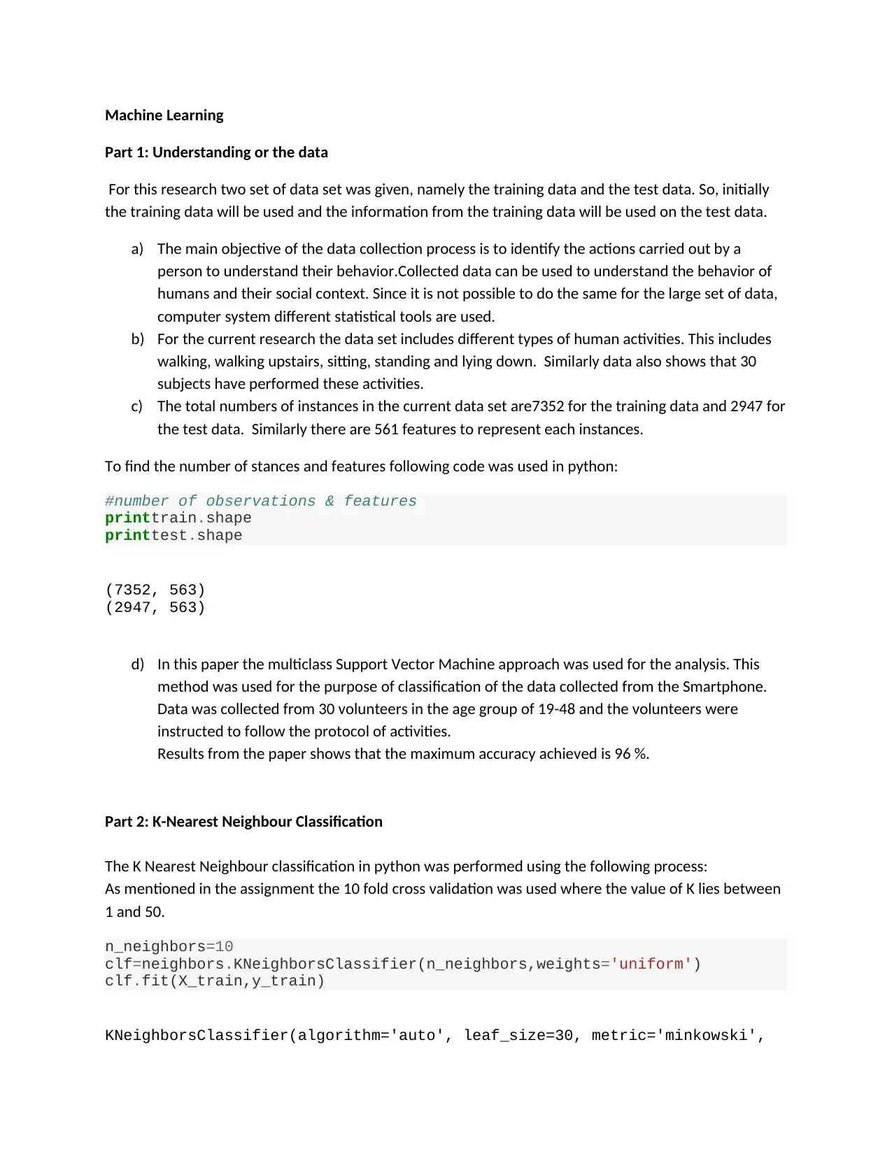
c) The total numbers of instances in the current data set are7352 for the training data and 2947 for
the test data. Similarly there are 561 features to represent each instances.
To find the number of stances and features following code was used in python:
#number of observations & features
printtrain.shape
printtest.shape
(7352, 563)
(2947, 563)
d) In this paper the multiclass Support Vector Machine approach was used for the analysis. This
method was used for the purpose of classification of the data collected from the Smartphone.
Data was collected from 30 volunteers in the age group of 19-48 and the volunteers were
instructed to follow the protocol of activities.
Results from the paper shows that the maximum accuracy achieved is 96 %.
Part 2: K-Nearest Neighbour Classification
The K Nearest Neighbour classification in python was performed using the following process:
As mentioned in the assignment the 10 fold cross validation was used where the value of K lies between
1 and 50.
n_neighbors=10
clf=neighbors.KNeighborsClassifier(n_neighbors,weights='uniform')
clf.fit(X_train,y_train)
KNeighborsClassifier(algorithm='auto', leaf_size=30, metric='minkowski',
Part 1: Understanding or the data
For this research two set of data set was given, namely the training data and the test data. So, initially
the training data will be used and the information from the training data will be used on the test data.
a) The main objective of the data collection process is to identify the actions carried out by a
person to understand their behavior.Collected data can be used to understand the behavior of
humans and their social context. Since it is not possible to do the same for the large set of data,
computer system different statistical tools are used.
b) For the current research the data set includes different types of human activities. This includes
walking, walking upstairs, sitting, standing and lying down. Similarly data also shows that 30
subjects have performed these activities.
c) The total numbers of instances in the current data set are7352 for the training data and 2947 for
the test data. Similarly there are 561 features to represent each instances.
To find the number of stances and features following code was used in python:
#number of observations & features
printtrain.shape
printtest.shape
(7352, 563)
(2947, 563)
d) In this paper the multiclass Support Vector Machine approach was used for the analysis. This
method was used for the purpose of classification of the data collected from the Smartphone.
Data was collected from 30 volunteers in the age group of 19-48 and the volunteers were
instructed to follow the protocol of activities.
Results from the paper shows that the maximum accuracy achieved is 96 %.
Part 2: K-Nearest Neighbour Classification
The K Nearest Neighbour classification in python was performed using the following process:
As mentioned in the assignment the 10 fold cross validation was used where the value of K lies between
1 and 50.
n_neighbors=10
clf=neighbors.KNeighborsClassifier(n_neighbors,weights='uniform')
clf.fit(X_train,y_train)
KNeighborsClassifier(algorithm='auto', leaf_size=30, metric='minkowski',
Paraphrase This Document
Need a fresh take? Get an instant paraphrase of this document with our AI Paraphraser
metric_params=None, n_neighbors=10, p=2, weights='uniform')
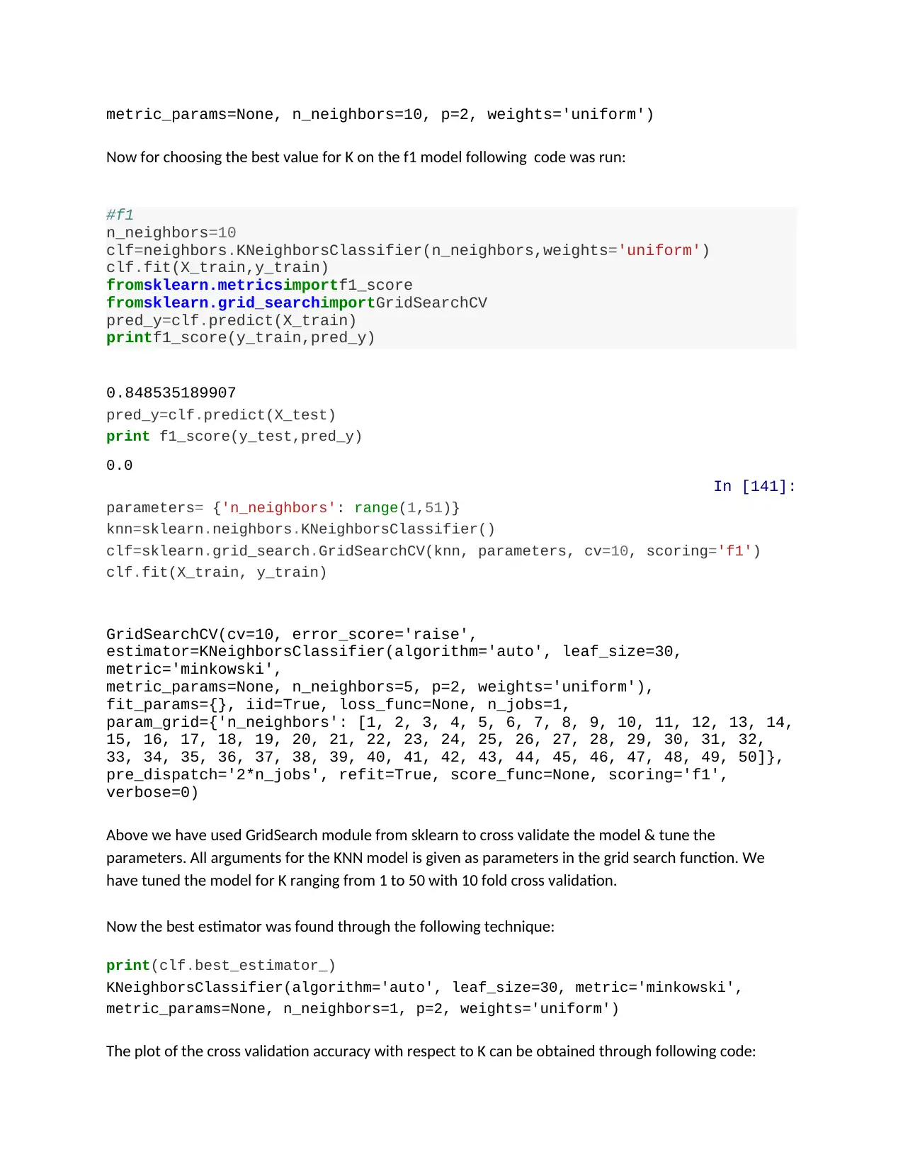
Now for choosing the best value for K on the f1 model following code was run:
#f1
n_neighbors=10
clf=neighbors.KNeighborsClassifier(n_neighbors,weights='uniform')
clf.fit(X_train,y_train)
fromsklearn.metricsimportf1_score
fromsklearn.grid_searchimportGridSearchCV
pred_y=clf.predict(X_train)
printf1_score(y_train,pred_y)
0.848535189907
pred_y=clf.predict(X_test)
print f1_score(y_test,pred_y)
0.0
In [141]:
parameters= {'n_neighbors': range(1,51)}
knn=sklearn.neighbors.KNeighborsClassifier()
clf=sklearn.grid_search.GridSearchCV(knn, parameters, cv=10, scoring='f1')
clf.fit(X_train, y_train)
GridSearchCV(cv=10, error_score='raise',
estimator=KNeighborsClassifier(algorithm='auto', leaf_size=30,
metric='minkowski',
metric_params=None, n_neighbors=5, p=2, weights='uniform'),
fit_params={}, iid=True, loss_func=None, n_jobs=1,
param_grid={'n_neighbors': [1, 2, 3, 4, 5, 6, 7, 8, 9, 10, 11, 12, 13, 14,
15, 16, 17, 18, 19, 20, 21, 22, 23, 24, 25, 26, 27, 28, 29, 30, 31, 32,
33, 34, 35, 36, 37, 38, 39, 40, 41, 42, 43, 44, 45, 46, 47, 48, 49, 50]},
pre_dispatch='2*n_jobs', refit=True, score_func=None, scoring='f1',
verbose=0)
Above we have used GridSearch module from sklearn to cross validate the model & tune the
parameters. All arguments for the KNN model is given as parameters in the grid search function. We
have tuned the model for K ranging from 1 to 50 with 10 fold cross validation.
Now the best estimator was found through the following technique:
print(clf.best_estimator_)
KNeighborsClassifier(algorithm='auto', leaf_size=30, metric='minkowski',
metric_params=None, n_neighbors=1, p=2, weights='uniform')
The plot of the cross validation accuracy with respect to K can be obtained through following code:
plot of cross validation accuracy with respect to K
neighbour_list=[]
mean_list=[]
std_list=[]
forneighbour,mean,stdinclf.grid_scores_:
neighbour_list.append(neighbour)
mean_list.append(mean)
std_list.append(np.std(std))
x=np.arange(1,len(neighbour_list)+1)
plt.plot(mean_list)
plt.show()
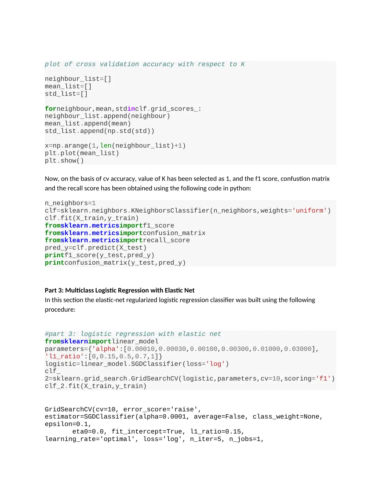
Now, on the basis of cv accuracy, value of K has been selected as 1, and the f1 score, confustion matrix
and the recall score has been obtained using the following code in python:
n_neighbors=1
clf=sklearn.neighbors.KNeighborsClassifier(n_neighbors,weights='uniform')
clf.fit(X_train,y_train)
fromsklearn.metricsimportf1_score
fromsklearn.metricsimportconfusion_matrix
fromsklearn.metricsimportrecall_score
pred_y=clf.predict(X_test)
printf1_score(y_test,pred_y)
printconfusion_matrix(y_test,pred_y)
Part 3: Multiclass Logistic Regression with Elastic Net
In this section the elastic-net regularized logistic regression classifier was built using the following
procedure:
#part 3: logistic regression with elastic net
fromsklearnimportlinear_model
parameters={'alpha':[0.00010,0.00030,0.00100,0.00300,0.01000,0.03000],
'l1_ratio':[0,0.15,0.5,0.7,1]}
logistic=linear_model.SGDClassifier(loss='log')
clf_
2=sklearn.grid_search.GridSearchCV(logistic,parameters,cv=10,scoring='f1')
clf_2.fit(X_train,y_train)
GridSearchCV(cv=10, error_score='raise',
estimator=SGDClassifier(alpha=0.0001, average=False, class_weight=None,
epsilon=0.1,
eta0=0.0, fit_intercept=True, l1_ratio=0.15,
learning_rate='optimal', loss='log', n_iter=5, n_jobs=1,
neighbour_list=[]
mean_list=[]
std_list=[]
forneighbour,mean,stdinclf.grid_scores_:
neighbour_list.append(neighbour)
mean_list.append(mean)
std_list.append(np.std(std))
x=np.arange(1,len(neighbour_list)+1)
plt.plot(mean_list)
plt.show()
Now, on the basis of cv accuracy, value of K has been selected as 1, and the f1 score, confustion matrix
and the recall score has been obtained using the following code in python:
n_neighbors=1
clf=sklearn.neighbors.KNeighborsClassifier(n_neighbors,weights='uniform')
clf.fit(X_train,y_train)
fromsklearn.metricsimportf1_score
fromsklearn.metricsimportconfusion_matrix
fromsklearn.metricsimportrecall_score
pred_y=clf.predict(X_test)
printf1_score(y_test,pred_y)
printconfusion_matrix(y_test,pred_y)
Part 3: Multiclass Logistic Regression with Elastic Net
In this section the elastic-net regularized logistic regression classifier was built using the following
procedure:
#part 3: logistic regression with elastic net
fromsklearnimportlinear_model
parameters={'alpha':[0.00010,0.00030,0.00100,0.00300,0.01000,0.03000],
'l1_ratio':[0,0.15,0.5,0.7,1]}
logistic=linear_model.SGDClassifier(loss='log')
clf_
2=sklearn.grid_search.GridSearchCV(logistic,parameters,cv=10,scoring='f1')
clf_2.fit(X_train,y_train)
GridSearchCV(cv=10, error_score='raise',
estimator=SGDClassifier(alpha=0.0001, average=False, class_weight=None,
epsilon=0.1,
eta0=0.0, fit_intercept=True, l1_ratio=0.15,
learning_rate='optimal', loss='log', n_iter=5, n_jobs=1,
⊘ This is a preview!⊘
Do you want full access?
Subscribe today to unlock all pages.
Trusted by 1+ million students worldwide
penalty='l2', power_t=0.5, random_state=None, shuffle=True,
verbose=0, warm_start=False),
fit_params={}, iid=True, loss_func=None, n_jobs=1,
param_grid={'alpha': [0.0001, 0.0003, 0.001, 0.003, 0.01, 0.03],
'l1_ratio': [0, 0.15, 0.5, 0.7, 1]},
pre_dispatch='2*n_jobs', refit=True, score_func=None, scoring='f1',
verbose=0)
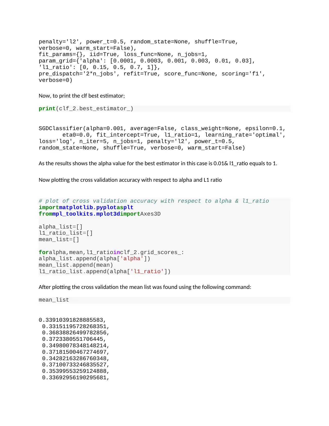
Now, to print the clf best estimator;
print(clf_2.best_estimator_)
SGDClassifier(alpha=0.001, average=False, class_weight=None, epsilon=0.1,
eta0=0.0, fit_intercept=True, l1_ratio=1, learning_rate='optimal',
loss='log', n_iter=5, n_jobs=1, penalty='l2', power_t=0.5,
random_state=None, shuffle=True, verbose=0, warm_start=False)
As the results shows the alpha value for the best estimator in this case is 0.01& l1_ratio equals to 1.
Now plotting the cross validation accuracy with respect to alpha and L1 ratio
# plot of cross validation accuracy with respect to alpha & l1_ratio
importmatplotlib.pyplotasplt
frommpl_toolkits.mplot3dimportAxes3D
alpha_list=[]
l1_ratio_list=[]
mean_list=[]
foralpha,mean,l1_ratioinclf_2.grid_scores_:
alpha_list.append(alpha['alpha'])
mean_list.append(mean)
l1_ratio_list.append(alpha['l1_ratio'])
After plotting the cross validation the mean list was found using the following command:
mean_list
0.33910391828885583,
0.33151195728268351,
0.36838826499782856,
0.3723380551706445,
0.34980078348148214,
0.37181500467274697,
0.34282163286760348,
0.37100733246835527,
0.35399553259124888,
0.33692956190295681,
verbose=0, warm_start=False),
fit_params={}, iid=True, loss_func=None, n_jobs=1,
param_grid={'alpha': [0.0001, 0.0003, 0.001, 0.003, 0.01, 0.03],
'l1_ratio': [0, 0.15, 0.5, 0.7, 1]},
pre_dispatch='2*n_jobs', refit=True, score_func=None, scoring='f1',
verbose=0)
Now, to print the clf best estimator;
print(clf_2.best_estimator_)
SGDClassifier(alpha=0.001, average=False, class_weight=None, epsilon=0.1,
eta0=0.0, fit_intercept=True, l1_ratio=1, learning_rate='optimal',
loss='log', n_iter=5, n_jobs=1, penalty='l2', power_t=0.5,
random_state=None, shuffle=True, verbose=0, warm_start=False)
As the results shows the alpha value for the best estimator in this case is 0.01& l1_ratio equals to 1.
Now plotting the cross validation accuracy with respect to alpha and L1 ratio
# plot of cross validation accuracy with respect to alpha & l1_ratio
importmatplotlib.pyplotasplt
frommpl_toolkits.mplot3dimportAxes3D
alpha_list=[]
l1_ratio_list=[]
mean_list=[]
foralpha,mean,l1_ratioinclf_2.grid_scores_:
alpha_list.append(alpha['alpha'])
mean_list.append(mean)
l1_ratio_list.append(alpha['l1_ratio'])
After plotting the cross validation the mean list was found using the following command:
mean_list
0.33910391828885583,
0.33151195728268351,
0.36838826499782856,
0.3723380551706445,
0.34980078348148214,
0.37181500467274697,
0.34282163286760348,
0.37100733246835527,
0.35399553259124888,
0.33692956190295681,
Paraphrase This Document
Need a fresh take? Get an instant paraphrase of this document with our AI Paraphraser
0.38480000325871044,
0.37995716060247431,
0.36685259732558362,
0.40035869664865514,
0.41256285464772563,
0.38741048125226984,
0.39636638270451074,
0.40270246206340748,
0.40973276063956238,
0.39437119591525394,
0.37771547432221053,
0.38141570211051662,
0.37322714834506421,
0.36745573664280251,
0.3619814496370759,
0.31989887743952466,
0.29392210987917289,
0.29589626225684945,
0.30317850296653653,
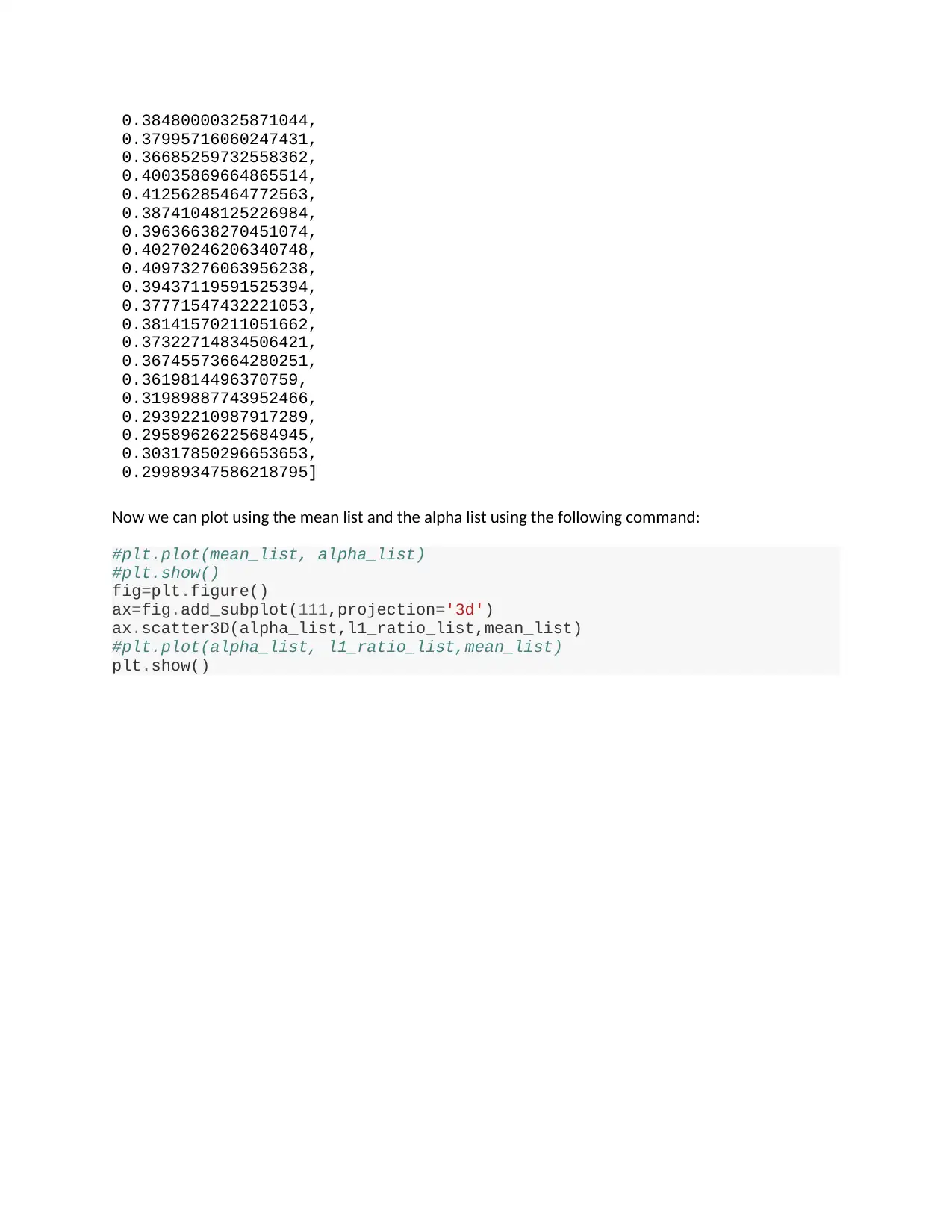
0.29989347586218795]
Now we can plot using the mean list and the alpha list using the following command:
#plt.plot(mean_list, alpha_list)
#plt.show()
fig=plt.figure()
ax=fig.add_subplot(111,projection='3d')
ax.scatter3D(alpha_list,l1_ratio_list,mean_list)
#plt.plot(alpha_list, l1_ratio_list,mean_list)
plt.show()
0.37995716060247431,
0.36685259732558362,
0.40035869664865514,
0.41256285464772563,
0.38741048125226984,
0.39636638270451074,
0.40270246206340748,
0.40973276063956238,
0.39437119591525394,
0.37771547432221053,
0.38141570211051662,
0.37322714834506421,
0.36745573664280251,
0.3619814496370759,
0.31989887743952466,
0.29392210987917289,
0.29589626225684945,
0.30317850296653653,
0.29989347586218795]
Now we can plot using the mean list and the alpha list using the following command:
#plt.plot(mean_list, alpha_list)
#plt.show()
fig=plt.figure()
ax=fig.add_subplot(111,projection='3d')
ax.scatter3D(alpha_list,l1_ratio_list,mean_list)
#plt.plot(alpha_list, l1_ratio_list,mean_list)
plt.show()
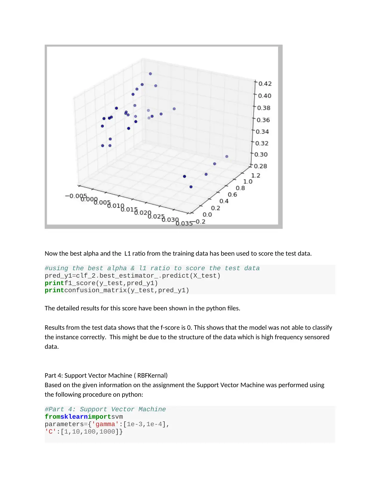
Now the best alpha and the L1 ratio from the training data has been used to score the test data.
#using the best alpha & l1 ratio to score the test data
pred_y1=clf_2.best_estimator_.predict(X_test)
printf1_score(y_test,pred_y1)
printconfusion_matrix(y_test,pred_y1)
The detailed results for this score have been shown in the python files.
Results from the test data shows that the f-score is 0. This shows that the model was not able to classify
the instance correctly. This might be due to the structure of the data which is high frequency sensored
data.
Part 4: Support Vector Machine ( RBFKernal)
Based on the given information on the assignment the Support Vector Machine was performed using
the following procedure on python:
#Part 4: Support Vector Machine
fromsklearnimportsvm
parameters={'gamma':[1e-3,1e-4],
'C':[1,10,100,1000]}
⊘ This is a preview!⊘
Do you want full access?
Subscribe today to unlock all pages.
Trusted by 1+ million students worldwide
clf_sv
m=sklearn.grid_search.GridSearchCV(svm.SVC(kernel='rbf'),parameters,cv=10,
scoring='f1')
clf_svm.fit(X_train,y_train)
GridSearchCV(cv=10, error_score='raise',
estimator=SVC(C=1.0, cache_size=200, class_weight=None, coef0=0.0,
degree=3, gamma=0.0,
kernel='rbf', max_iter=-1, probability=False, random_state=None,
shrinking=True, tol=0.001, verbose=False),
fit_params={}, iid=True, loss_func=None, n_jobs=1,
param_grid={'C': [1, 10, 100, 1000], 'gamma': [0.001, 0.0001]},
pre_dispatch='2*n_jobs', refit=True, score_func=None, scoring='f1',
verbose=0)
Now, finding the classification of SVM best estimator :
clf_svm.best_estimator_
SVC(C=100, cache_size=200, class_weight=None, coef0=0.0, degree=3,
gamma=0.001, kernel='rbf', max_iter=-1, probability=False,
random_state=None, shrinking=True, tol=0.001, verbose=False)
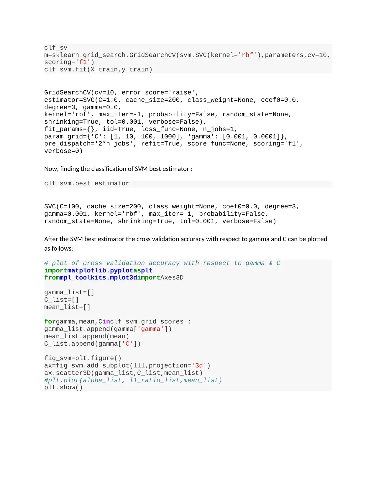
After the SVM best estimator the cross validation accuracy with respect to gamma and C can be plotted
as follows:
# plot of cross validation accuracy with respect to gamma & C
importmatplotlib.pyplotasplt
frommpl_toolkits.mplot3dimportAxes3D
gamma_list=[]
C_list=[]
mean_list=[]
forgamma,mean,Cinclf_svm.grid_scores_:
gamma_list.append(gamma['gamma'])
mean_list.append(mean)
C_list.append(gamma['C'])
fig_svm=plt.figure()
ax=fig_svm.add_subplot(111,projection='3d')
ax.scatter3D(gamma_list,C_list,mean_list)
#plt.plot(alpha_list, l1_ratio_list,mean_list)
plt.show()
m=sklearn.grid_search.GridSearchCV(svm.SVC(kernel='rbf'),parameters,cv=10,
scoring='f1')
clf_svm.fit(X_train,y_train)
GridSearchCV(cv=10, error_score='raise',
estimator=SVC(C=1.0, cache_size=200, class_weight=None, coef0=0.0,
degree=3, gamma=0.0,
kernel='rbf', max_iter=-1, probability=False, random_state=None,
shrinking=True, tol=0.001, verbose=False),
fit_params={}, iid=True, loss_func=None, n_jobs=1,
param_grid={'C': [1, 10, 100, 1000], 'gamma': [0.001, 0.0001]},
pre_dispatch='2*n_jobs', refit=True, score_func=None, scoring='f1',
verbose=0)
Now, finding the classification of SVM best estimator :
clf_svm.best_estimator_
SVC(C=100, cache_size=200, class_weight=None, coef0=0.0, degree=3,
gamma=0.001, kernel='rbf', max_iter=-1, probability=False,
random_state=None, shrinking=True, tol=0.001, verbose=False)
After the SVM best estimator the cross validation accuracy with respect to gamma and C can be plotted
as follows:
# plot of cross validation accuracy with respect to gamma & C
importmatplotlib.pyplotasplt
frommpl_toolkits.mplot3dimportAxes3D
gamma_list=[]
C_list=[]
mean_list=[]
forgamma,mean,Cinclf_svm.grid_scores_:
gamma_list.append(gamma['gamma'])
mean_list.append(mean)
C_list.append(gamma['C'])
fig_svm=plt.figure()
ax=fig_svm.add_subplot(111,projection='3d')
ax.scatter3D(gamma_list,C_list,mean_list)
#plt.plot(alpha_list, l1_ratio_list,mean_list)
plt.show()
Paraphrase This Document
Need a fresh take? Get an instant paraphrase of this document with our AI Paraphraser
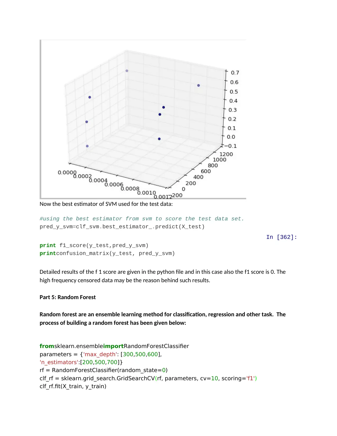
Now the best estimator of SVM used for the test data:
#using the best estimator from svm to score the test data set.
pred_y_svm=clf_svm.best_estimator_.predict(X_test)
In [362]:
print f1_score(y_test,pred_y_svm)
printconfusion_matrix(y_test, pred_y_svm)
Detailed results of the f 1 score are given in the python file and in this case also the f1 score is 0. The
high frequency censored data may be the reason behind such results.
Part 5: Random Forest
Random forest are an ensemble learning method for classification, regression and other task. The
process of building a random forest has been given below:
fromsklearn.ensembleimportRandomForestClassifier
parameters = {'max_depth': [300,500,600],
'n_estimators':[200,500,700]}
rf = RandomForestClassifier(random_state=0)
clf_rf = sklearn.grid_search.GridSearchCV(rf, parameters, cv=10, scoring='f1')
clf_rf.fit(X_train, y_train)
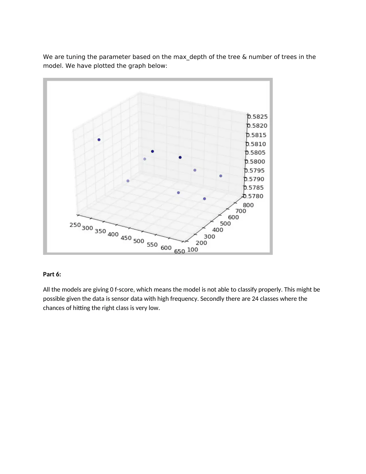
We are tuning the parameter based on the max_depth of the tree & number of trees in the
model. We have plotted the graph below:
Part 6:
All the models are giving 0 f-score, which means the model is not able to classify properly. This might be
possible given the data is sensor data with high frequency. Secondly there are 24 classes where the
chances of hitting the right class is very low.
⊘ This is a preview!⊘
Do you want full access?
Subscribe today to unlock all pages.
Trusted by 1+ million students worldwide
1 out of 9

Your All-in-One AI-Powered Toolkit for Academic Success.
+13062052269
info@desklib.com
Available 24*7 on WhatsApp / Email
![[object Object]](/_next/static/media/star-bottom.7253800d.svg)
Unlock your academic potential
Copyright © 2020–2026 A2Z Services. All Rights Reserved. Developed and managed by ZUCOL.