Modeling and Predicting NYC Real Estate Sales Prices: Project Report
VerifiedAdded on 2022/08/24
|21
|5450
|14
Project
AI Summary
This project focuses on predicting real estate prices in New York City using machine learning techniques. The student utilized a dataset containing sales information of various properties across five boroughs over a 12-month period. The analysis employed an artificial neural network model using deep learning, specifically the Keras Regressor algorithm, to train and test the data. The project includes data exploration, visualization, and model development using Keras layers and TensorFlow in the backend. The report provides an executive summary, introduction, discussion of the dataset, the proposed price prediction model, and conclusions. The model's performance and predictions are evaluated, with the aim of identifying patterns and insights within the dataset. The project highlights the effectiveness of deep learning in predicting real estate prices and provides a comprehensive analysis of the data, including the impact of different features on sales prices.
Running head: MODELING & COMPUTING TECHNIQUES
Modeling & Computing Techniques
Students Name:
Student ID:
University Name:
Paper code:
Modeling & Computing Techniques
Students Name:
Student ID:
University Name:
Paper code:
Paraphrase This Document
Need a fresh take? Get an instant paraphrase of this document with our AI Paraphraser
2MODELING & COMPUTING TECHNIQUES
Executive Summary
Machine learning and Artificial Intelligence is considered to be one of the leading and powerful
technologies used in the recent world. The most important part is that human’s haven’t seen the
full potential of such technologies. This is because the system has the ability to learn
automatically from historical data and from past experience. Machine learning technology are
generally used to transform information into knowledge. Machine learning models are used to
gather useful information and the hidden patterns inside the data and make decisions based on
the data with minimum human involvement.
The dataset used in the analysis contains information of each and every building like
home, apartment etc. which are sold in the New York City property market over the period of 12
months. The dataset contains information of five different places. A total number of 84548
numbers of information are present into the data file.
The model used for classifying the sales is artificial neural network model using deep
learning. Basically Keras Regressor algorithm is used to train the training dataset and will be
tested over the tested dataset as how well the classifier classified the target variable values. It can
be said that deep learning or the neural network models provides better prediction rate as
compare to other model.
In the analysis a deep thorough analysis, data exploration, visualization and at the end
prediction has been performed to get in-depth knowledge of the dataset. Proper machine learning
model with keras layers and tensorflow in the backend has been developed using neural network
techniques. At the end a conclusion will be concluded on how the model predicts the sale price
and different hidden patterns and information will be drawn in the end.
3MODELING & COMPUTING TECHNIQUES
Table of Contents
Executive Summary.........................................................................................................................2
Introduction......................................................................................................................................4
Discussion........................................................................................................................................4
Introduction and observation of the dataset.................................................................................4
The proposed model for price prediction.....................................................................................8
Conclusion.....................................................................................................................................10
References......................................................................................................................................11
Appendix........................................................................................................................................13
⊘ This is a preview!⊘
Do you want full access?
Subscribe today to unlock all pages.
Trusted by 1+ million students worldwide
4MODELING & COMPUTING TECHNIQUES
Introduction
Machine learning and Artificial Intelligence is considered to be one of the leading and
powerful technologies used in the recent world (Alpaydin, 2020). The most important part is that
human’s haven’t seen the full potential of such technologies. This is because the system has the
ability to learn automatically from historical data and from past experience. Machine learning
technology are generally used to transform information into knowledge (Bishop, 2006). Machine
learning models are used to find the hidden patterns inside the data and make decisions based on
the data with minimum human involvement (Moolayil, Moolayil & John, 2019). Mainly there
are 2 types of machine learning algorithm categories mainly supervised and unsupervised
learning (Brownlee, 2016).
In supervised learning the inputs of the dataset is known and the dataset contains labelled
data with known output, whereas in unsupervised learning the input is known but the dataset
contains, un-labelled data with unknown outputs (Campesato, 2020). In this analysis the target
variable is the sale price attribute and the goal is to predict the sales price using artificial neural
network using deep learning methods (Chernick, 1998).
Deep learning is another field or it can be said that it is a subpart of machine learning
which consist of network based layers and capable of learning from the unsupervised data which
are generally unstructured and unlabeled (Daniel, 2013). There are different kinds of layers used
to build a neural network model. For this analysis only dense layer has been used to build the
artificial neural network model (Dietterich, 1997).
The accuracy and the performance of the models also depends on the data. If the data
contains more missing values or null values then the model will not be able to classify properly
as the data is not a good fit for the model (Géron, 2019). The more cleanly the data the more
acutely the model will classify the target variables. It has been seen that using deep learning
more accurate result has been observed instead of using older learning algorithms (Mitchell,
1997).
Discussion
Introduction and observation of the dataset
Exploring the attributes of the dataset:
1. BOROUGH: The Borough attribute consist of 5 different classes which are basically five
location where properties have been sold which are basically, 1 for 'Manhattan', 2 for
'Bronx', 3 for 'Brooklyn', 4 for 'Queens' and 5 for 'Staten Island' and these should be
considered to be categorical values.
2. NEIGHBORHOOD: This attribute tells the neighborhood name for the particular
properties. The name is given by the department of finance assessors also the name is
similar to the name of the Finance designates. Also it can be seen that there may be few
differences in the neighborhood attributes and few sub- neighborhood might not be
include also with respect to the value of the attribute the attribute will be categorical.
Paraphrase This Document
Need a fresh take? Get an instant paraphrase of this document with our AI Paraphraser
5MODELING & COMPUTING TECHNIQUES
3. BUILDING CLASS CATEGORY: This attribute is used to identify similar properties of
the Rolling sales files without having look into individual building classes (Norris, 2020).
The data and files are been store by the Neighborhood, Block, Borough, Building Class
Category and lot. Also the values of the attribute are said to be categorical.
4. TAX CLASS AT PRESENT, there consist of 4 tax classes mainly, 1,2,3 and 4 which are
assigned to each property of the city which are totally based on the use of the property
also this attribute consist of categorical values.
Class 1: This includes most of the attribute which are mainly one, two or three family
houses with such small store or offices, vacant lands are used for residential use and most
important there should not be any three stories.
Class 2: This shoes the properties which are generally primarily residents mainly the
condominiums and the cooperatives.
Class 3: This includes the properties which are generally equipped and owned by
telephones, gas and electric companies.
Class 4: This includes which are not included in the class1, class2 and class3 mainly the
factories, garage, offices, warehouses and many more.
5. BLOCK and LOT: Here the tax block is termed to be as the sub division of borough
attributes. The block and lot distinguishes one unit of real property from another, such as
the different condominiums in a single building (Yao, 1999). The tax lot represent the
unique location of the properties which is generally a subdivision of a tax block. Also
making it categorical doesn’t make any sense as there are 11k unique blocks available in
the dataset. Hence both block and lot will be uses as numerical attributes for the analysis
purpose.
6. BUILDING CLASS AT PRESENT: This attribute is used for describing the constructive
use of properties. The first letter describe the individual class of the properties for
example “A” signifies one-family homes, “O” signifies office buildings. “R” signifies
condominiums (Michie & Spiegelhalter, 1994). For the second position some numbers
are been added with the previous examples which can be written in the form of “A0” is a
Cape Cod style one family home, “O4” is a tower type office building and “R5” is a
commercial condominium unit. The values of the attribute will be categorical as there
will be unique code given for the properties.
7. ADDRESS: The address basically consist of the street address for the property which are
been listed in the sales file. Apartment number are use in the address field for the coop
sale.
8. ZIP CODE: It tell the postal code for each property. This variable should be categorical.
9. RESIDENTIAL UNITS: This attributes tell the total number of residential unit which are
listed for each property. This variable should be numeric.
10. COMMERCIAL UNITS: This attributes tell the total number of commercial unit which
are listed for each property. This variable should be numeric.
6MODELING & COMPUTING TECHNIQUES
11. TOTAL UNITS: This attribute tell the total number of units that are listed for each
property. This variable should be numeric
12. LAND SQUARE FEET: It consist of the total land area for particular property measure
in square feet. This attribute should be numeric
13. GROSS SQUARE FEET : It is the measurement of the total measured area including the
exterior surface then the outside wall of the building also the outside space are also taken
to consideration. This attribute will be numeric.
8. YEAR BUILT: The attribute indicates the year when the property was built also the
values of the attributes will be categorical.
9. TAX CLASS AT TIME OF SALE and BUILDING CLASS AT TIME OF SALE. Both
these attributes will be categorical.
10. SALE PRICE: This variable should be numeric.
11. SALE DATE: This variable should be data time. However, we can save the "year" or
"month" part as a new categorical variable.
12. EASEMENT: This attributes indicates some right which needs to be followed, it depicts
some entity which have limited rights to use another’s property.
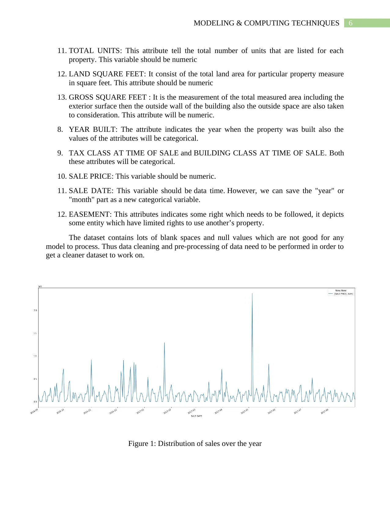
The dataset contains lots of blank spaces and null values which are not good for any
model to process. Thus data cleaning and pre-processing of data need to be performed in order to
get a cleaner dataset to work on.
Figure 1: Distribution of sales over the year
11. TOTAL UNITS: This attribute tell the total number of units that are listed for each
property. This variable should be numeric
12. LAND SQUARE FEET: It consist of the total land area for particular property measure
in square feet. This attribute should be numeric
13. GROSS SQUARE FEET : It is the measurement of the total measured area including the
exterior surface then the outside wall of the building also the outside space are also taken
to consideration. This attribute will be numeric.
8. YEAR BUILT: The attribute indicates the year when the property was built also the
values of the attributes will be categorical.
9. TAX CLASS AT TIME OF SALE and BUILDING CLASS AT TIME OF SALE. Both
these attributes will be categorical.
10. SALE PRICE: This variable should be numeric.
11. SALE DATE: This variable should be data time. However, we can save the "year" or
"month" part as a new categorical variable.
12. EASEMENT: This attributes indicates some right which needs to be followed, it depicts
some entity which have limited rights to use another’s property.
The dataset contains lots of blank spaces and null values which are not good for any
model to process. Thus data cleaning and pre-processing of data need to be performed in order to
get a cleaner dataset to work on.
Figure 1: Distribution of sales over the year
⊘ This is a preview!⊘
Do you want full access?
Subscribe today to unlock all pages.
Trusted by 1+ million students worldwide
7MODELING & COMPUTING TECHNIQUES
Figure 1 represents the trend of sale price over the specific time period.
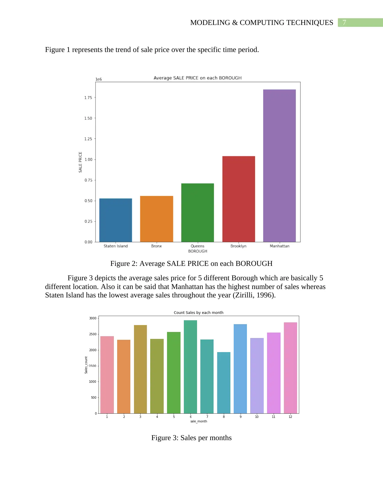
Figure 2: Average SALE PRICE on each BOROUGH
Figure 3 depicts the average sales price for 5 different Borough which are basically 5
different location. Also it can be said that Manhattan has the highest number of sales whereas
Staten Island has the lowest average sales throughout the year (Zirilli, 1996).
Figure 3: Sales per months
Figure 1 represents the trend of sale price over the specific time period.
Figure 2: Average SALE PRICE on each BOROUGH
Figure 3 depicts the average sales price for 5 different Borough which are basically 5
different location. Also it can be said that Manhattan has the highest number of sales whereas
Staten Island has the lowest average sales throughout the year (Zirilli, 1996).
Figure 3: Sales per months
Paraphrase This Document
Need a fresh take? Get an instant paraphrase of this document with our AI Paraphraser
8MODELING & COMPUTING TECHNIQUES
There are different analysis which can be used to find different patterns and useful
information from any dataset. Figure 3 shows the sales count for the 12 months of all the
Borough in total.
The dataset contains null values, missing values and duplicate values which needs to be
remove to get close insight of the data (Zurada, 1992). Also using correlation matrix other
important less attributes were deleted which doesn’t have such importance in the dataset (Gulli &
Pal, 2017).
After different analysis and visualization it’s now time to do different tweaks to the pre-
processed data and split the data into training and testing set which will be used to feed the
model (Jain, Mao & Mohiuddin, 1996).
The proposed model for price prediction
One of the most popular libraries which is used for deep learning is known as Keras, it is
widely to build neural network due to its simplicity and ease of use (Hassoun, 1995). Keras is a
high-level Python neural networks library that runs on top of the TensorFlow (Ketkar, 2017). In
the backend of the neural network tensorflow has been used during the model builup
(Limsombunchai, 2004).
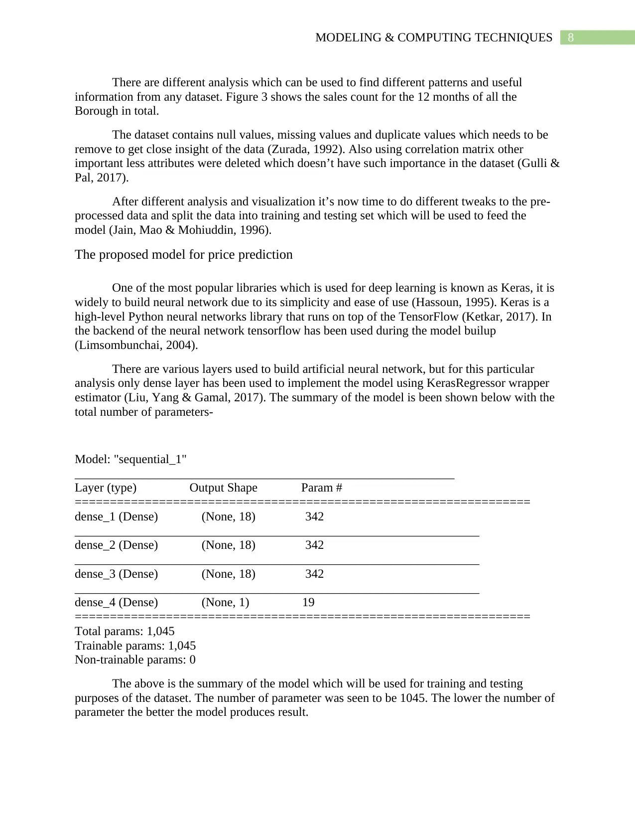
There are various layers used to build artificial neural network, but for this particular
analysis only dense layer has been used to implement the model using KerasRegressor wrapper
estimator (Liu, Yang & Gamal, 2017). The summary of the model is been shown below with the
total number of parameters-
Model: "sequential_1"
_____________________________________________________________
Layer (type) Output Shape Param #
=================================================================
dense_1 (Dense) (None, 18) 342
_________________________________________________________________
dense_2 (Dense) (None, 18) 342
_________________________________________________________________
dense_3 (Dense) (None, 18) 342
_________________________________________________________________
dense_4 (Dense) (None, 1) 19
=================================================================
Total params: 1,045
Trainable params: 1,045
Non-trainable params: 0
The above is the summary of the model which will be used for training and testing
purposes of the dataset. The number of parameter was seen to be 1045. The lower the number of
parameter the better the model produces result.
There are different analysis which can be used to find different patterns and useful
information from any dataset. Figure 3 shows the sales count for the 12 months of all the
Borough in total.
The dataset contains null values, missing values and duplicate values which needs to be
remove to get close insight of the data (Zurada, 1992). Also using correlation matrix other
important less attributes were deleted which doesn’t have such importance in the dataset (Gulli &
Pal, 2017).
After different analysis and visualization it’s now time to do different tweaks to the pre-
processed data and split the data into training and testing set which will be used to feed the
model (Jain, Mao & Mohiuddin, 1996).
The proposed model for price prediction
One of the most popular libraries which is used for deep learning is known as Keras, it is
widely to build neural network due to its simplicity and ease of use (Hassoun, 1995). Keras is a
high-level Python neural networks library that runs on top of the TensorFlow (Ketkar, 2017). In
the backend of the neural network tensorflow has been used during the model builup
(Limsombunchai, 2004).
There are various layers used to build artificial neural network, but for this particular
analysis only dense layer has been used to implement the model using KerasRegressor wrapper
estimator (Liu, Yang & Gamal, 2017). The summary of the model is been shown below with the
total number of parameters-
Model: "sequential_1"
_____________________________________________________________
Layer (type) Output Shape Param #
=================================================================
dense_1 (Dense) (None, 18) 342
_________________________________________________________________
dense_2 (Dense) (None, 18) 342
_________________________________________________________________
dense_3 (Dense) (None, 18) 342
_________________________________________________________________
dense_4 (Dense) (None, 1) 19
=================================================================
Total params: 1,045
Trainable params: 1,045
Non-trainable params: 0
The above is the summary of the model which will be used for training and testing
purposes of the dataset. The number of parameter was seen to be 1045. The lower the number of
parameter the better the model produces result.
9MODELING & COMPUTING TECHNIQUES
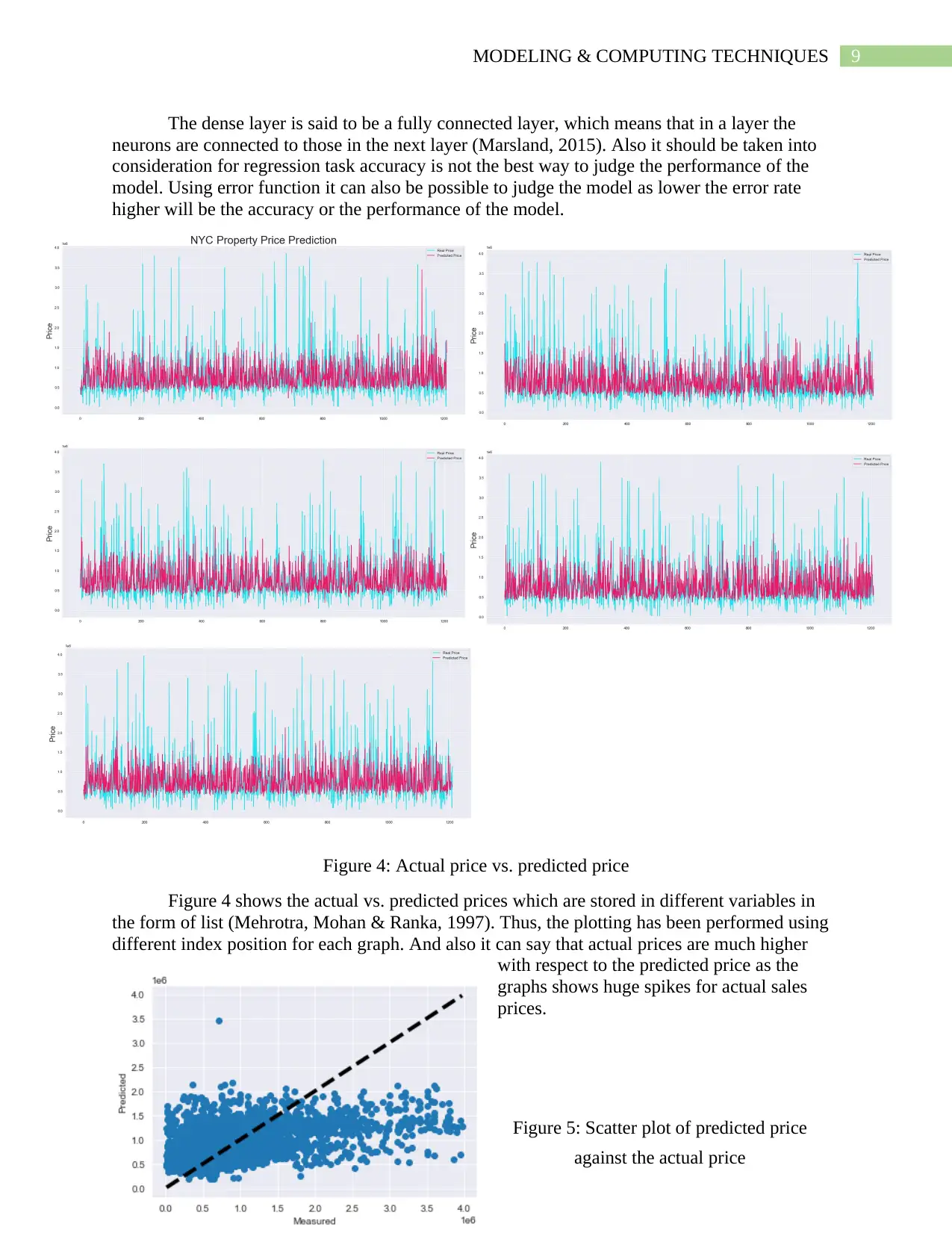
The dense layer is said to be a fully connected layer, which means that in a layer the
neurons are connected to those in the next layer (Marsland, 2015). Also it should be taken into
consideration for regression task accuracy is not the best way to judge the performance of the
model. Using error function it can also be possible to judge the model as lower the error rate
higher will be the accuracy or the performance of the model.
Figure 4: Actual price vs. predicted price
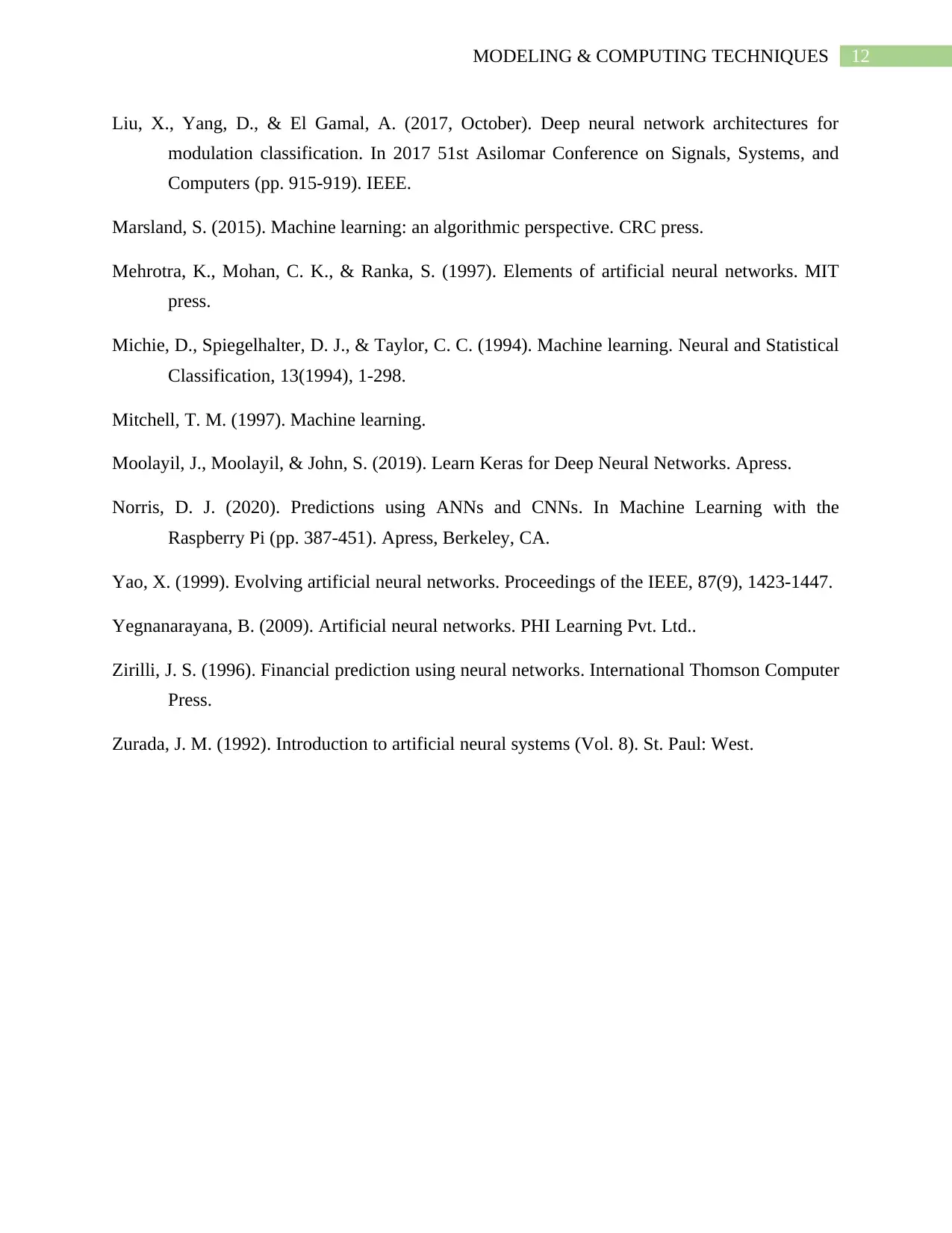
Figure 4 shows the actual vs. predicted prices which are stored in different variables in
the form of list (Mehrotra, Mohan & Ranka, 1997). Thus, the plotting has been performed using
different index position for each graph. And also it can say that actual prices are much higher
with respect to the predicted price as the
graphs shows huge spikes for actual sales
prices.
Figure 5: Scatter plot of predicted price
against the actual price
The dense layer is said to be a fully connected layer, which means that in a layer the
neurons are connected to those in the next layer (Marsland, 2015). Also it should be taken into
consideration for regression task accuracy is not the best way to judge the performance of the
model. Using error function it can also be possible to judge the model as lower the error rate
higher will be the accuracy or the performance of the model.
Figure 4: Actual price vs. predicted price
Figure 4 shows the actual vs. predicted prices which are stored in different variables in
the form of list (Mehrotra, Mohan & Ranka, 1997). Thus, the plotting has been performed using
different index position for each graph. And also it can say that actual prices are much higher
with respect to the predicted price as the
graphs shows huge spikes for actual sales
prices.
Figure 5: Scatter plot of predicted price
against the actual price
⊘ This is a preview!⊘
Do you want full access?
Subscribe today to unlock all pages.
Trusted by 1+ million students worldwide
10MODELING & COMPUTING TECHNIQUES
Conclusion
From the above analysis and result it can be concluded that the dataset given is not a
clean dataset due to which many data cleaning and pre-processing of data has been performed.
Also different finding have been shown using various visualization function. Although the data
was not a good one to feed into any machine learning model in spite a KerasRegressor with
dense layer has been built to check the predicted sales price.
Also accuracy measurement for regression algorithm is not a good choice to go in spite
looking at the error rate it can also be told how well the model has performed. In the discussion
portion of the report various conclusion has been made with respect to different graphs. Various
analysis has been performed to get in-depth knowledge of the dataset.
Some of the major improvement is to use cross validation after the model has been built
and after performing the estimator. Also error rates need to be calculated in order to see how well
the process reduced the error rate from previous. Also different layers need to be built to test how
well the newly designed model works with the dataset.
Paraphrase This Document
Need a fresh take? Get an instant paraphrase of this document with our AI Paraphraser
11MODELING & COMPUTING TECHNIQUES
References
Alpaydin, E. (2020). Introduction to machine learning. MIT press.
Bishop, C. M. (2006). Pattern recognition and machine learning. springer.
Brownlee, J. (2016). Deep learning with Python: develop deep learning models on Theano and
TensorFlow using Keras. Machine Learning Mastery.
Campesato, O. (2020). Artificial Intelligence, Machine Learning, and Deep Learning. Stylus
Publishing, LLC.
Chernick, H. (1998). Fiscal capacity in New York: The city versus the region. National Tax
Journal, 531-540.
Daniel, G. (2013). Principles of artificial neural networks (Vol. 7). World Scientific.
Dietterich, T. G. (1997). Machine-learning research. AI magazine, 18(4), 97-97.
Géron, A. (2019). Hands-On Machine Learning with Scikit-Learn, Keras, and TensorFlow:
Concepts, Tools, and Techniques to Build Intelligent Systems. O'Reilly Media.
Gulli, A., & Pal, S. (2017). Deep learning with Keras. Packt Publishing Ltd.
Hassoun, M. H. (1995). Fundamentals of artificial neural networks. MIT press.
Jain, A. K., Mao, J., & Mohiuddin, K. M. (1996). Artificial neural networks: A tutorial.
Computer, 29(3), 31-44.
Ketkar, N. (2017). Introduction to keras. In Deep learning with Python (pp. 97-111). Apress,
Berkeley, CA.
Limsombunchai, V. (2004, June). House price prediction: hedonic price model vs. artificial
neural network. In New Zealand agricultural and resource economics society conference
(pp. 25-26).
12MODELING & COMPUTING TECHNIQUES
Liu, X., Yang, D., & El Gamal, A. (2017, October). Deep neural network architectures for
modulation classification. In 2017 51st Asilomar Conference on Signals, Systems, and
Computers (pp. 915-919). IEEE.
Marsland, S. (2015). Machine learning: an algorithmic perspective. CRC press.
Mehrotra, K., Mohan, C. K., & Ranka, S. (1997). Elements of artificial neural networks. MIT
press.
Michie, D., Spiegelhalter, D. J., & Taylor, C. C. (1994). Machine learning. Neural and Statistical
Classification, 13(1994), 1-298.
Mitchell, T. M. (1997). Machine learning.
Moolayil, J., Moolayil, & John, S. (2019). Learn Keras for Deep Neural Networks. Apress.
Norris, D. J. (2020). Predictions using ANNs and CNNs. In Machine Learning with the
Raspberry Pi (pp. 387-451). Apress, Berkeley, CA.
Yao, X. (1999). Evolving artificial neural networks. Proceedings of the IEEE, 87(9), 1423-1447.
Yegnanarayana, B. (2009). Artificial neural networks. PHI Learning Pvt. Ltd..
Zirilli, J. S. (1996). Financial prediction using neural networks. International Thomson Computer
Press.
Zurada, J. M. (1992). Introduction to artificial neural systems (Vol. 8). St. Paul: West.
⊘ This is a preview!⊘
Do you want full access?
Subscribe today to unlock all pages.
Trusted by 1+ million students worldwide
1 out of 21
Related Documents


Your All-in-One AI-Powered Toolkit for Academic Success.
+13062052269
info@desklib.com
Available 24*7 on WhatsApp / Email
![[object Object]](/_next/static/media/star-bottom.7253800d.svg)
Unlock your academic potential
Copyright © 2020–2026 A2Z Services. All Rights Reserved. Developed and managed by ZUCOL.