Machine Learning for Student Success: ABCEU Project Report Analysis
VerifiedAdded on 2023/01/11
|23
|5105
|51
Report
AI Summary
This report presents an analysis of student data from ABC Universal Education (ABCEU) to predict pass rates using machine learning techniques. The objective is to identify factors that significantly influence student success. The analysis employs a data-driven approach, utilizing machine learning algorithms including Decision Trees, Random Forest, and Generalized Linear Models (GLM). After data exploration and feature selection, the models are implemented in R, and their performance is evaluated using metrics such as accuracy, sensitivity, specificity, and the confusion matrix. The Random Forest model demonstrates the highest accuracy. The report includes an executive summary, data exploration, feature selection, model selection, and validation. The findings provide insights into the most relevant factors determining student pass rates, offering ABCEU actionable recommendations to improve student outcomes.
1
Executive Summary
Objective
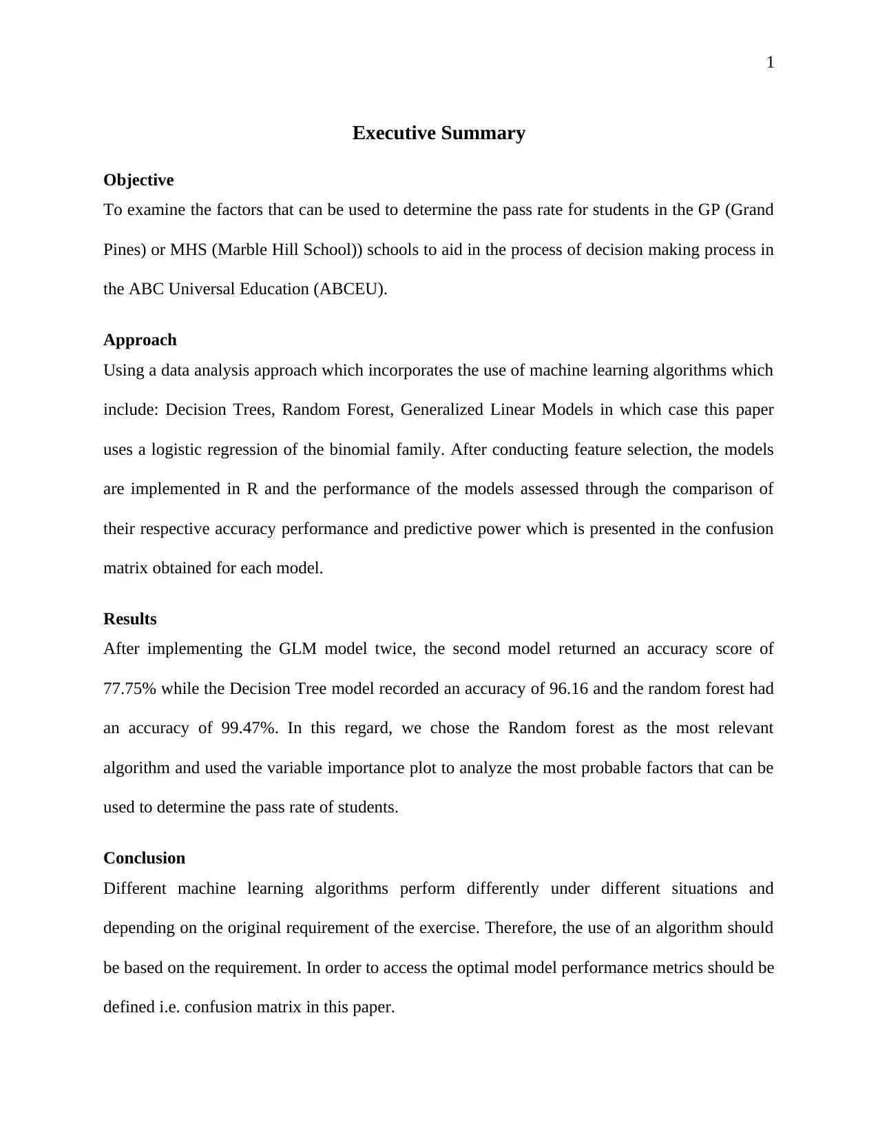
To examine the factors that can be used to determine the pass rate for students in the GP (Grand
Pines) or MHS (Marble Hill School)) schools to aid in the process of decision making process in
the ABC Universal Education (ABCEU).
Approach
Using a data analysis approach which incorporates the use of machine learning algorithms which
include: Decision Trees, Random Forest, Generalized Linear Models in which case this paper
uses a logistic regression of the binomial family. After conducting feature selection, the models
are implemented in R and the performance of the models assessed through the comparison of
their respective accuracy performance and predictive power which is presented in the confusion
matrix obtained for each model.
Results
After implementing the GLM model twice, the second model returned an accuracy score of
77.75% while the Decision Tree model recorded an accuracy of 96.16 and the random forest had
an accuracy of 99.47%. In this regard, we chose the Random forest as the most relevant
algorithm and used the variable importance plot to analyze the most probable factors that can be
used to determine the pass rate of students.
Conclusion
Different machine learning algorithms perform differently under different situations and
depending on the original requirement of the exercise. Therefore, the use of an algorithm should
be based on the requirement. In order to access the optimal model performance metrics should be
defined i.e. confusion matrix in this paper.
Paraphrase This Document
Need a fresh take? Get an instant paraphrase of this document with our AI Paraphraser
2
Data Exploration and Feature Selection
Data Exploration
In machine learning, the very basic objective is to try and gain an understanding of the data that
is presented to the analyst. In this respect, the question of what really is in the data crops up
crops up. Most often, machine leaning algorithms have been proven effective in offering a means
as to which the analyst can use to answer such a question (Sutton, 2018). Some of the popular
data exploration methods include visual data exploration and descriptive data analytics both of
which are used to gain understanding of factors such as the distribution of data attributes,
outliers, normality of the data and determine which factors are correlated, etcetera. In this paper
we will only explore univariate distributions of the data to examine: measures of location and
spread, asymmetry, outliers, missing data and gaps.
Descriptive
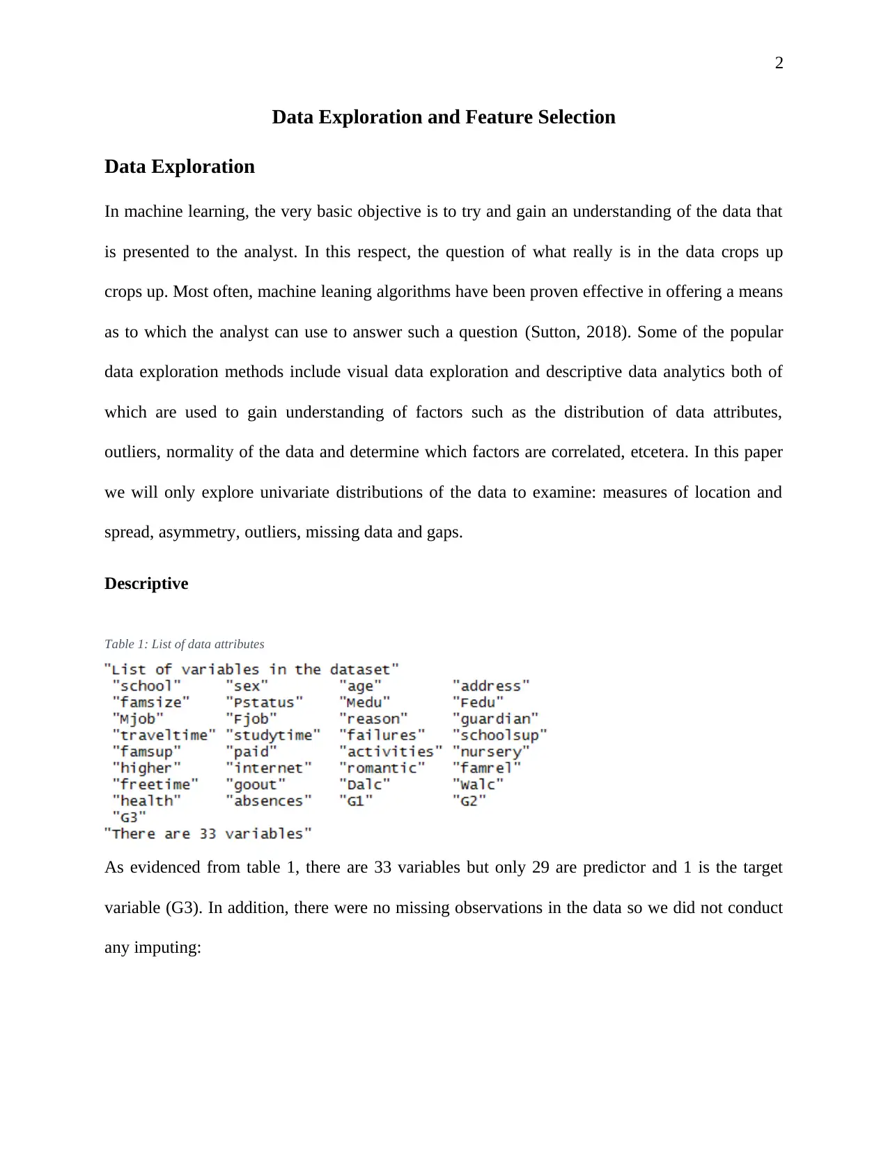
Table 1: List of data attributes
As evidenced from table 1, there are 33 variables but only 29 are predictor and 1 is the target
variable (G3). In addition, there were no missing observations in the data so we did not conduct
any imputing:
3
Correlation
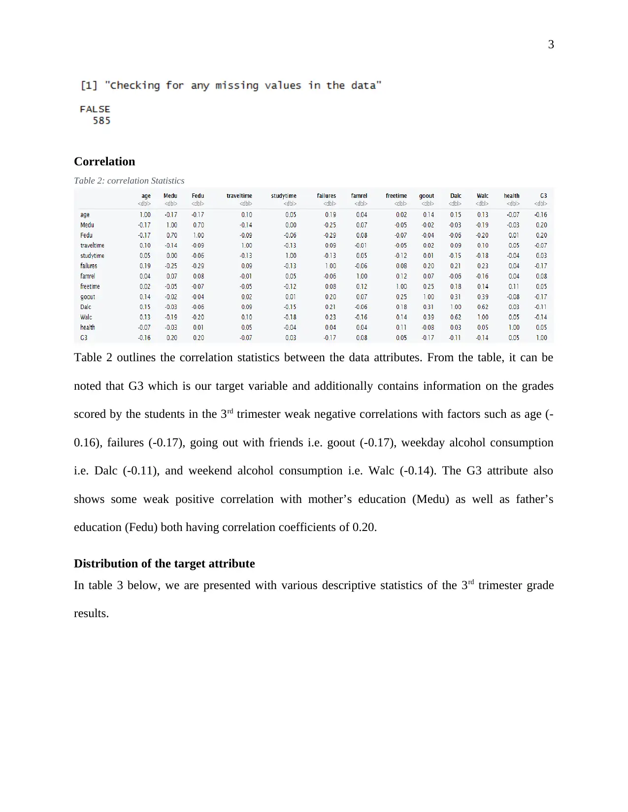
Table 2: correlation Statistics
Table 2 outlines the correlation statistics between the data attributes. From the table, it can be
noted that G3 which is our target variable and additionally contains information on the grades
scored by the students in the 3rd trimester weak negative correlations with factors such as age (-
0.16), failures (-0.17), going out with friends i.e. goout (-0.17), weekday alcohol consumption
i.e. Dalc (-0.11), and weekend alcohol consumption i.e. Walc (-0.14). The G3 attribute also
shows some weak positive correlation with mother’s education (Medu) as well as father’s
education (Fedu) both having correlation coefficients of 0.20.
Distribution of the target attribute
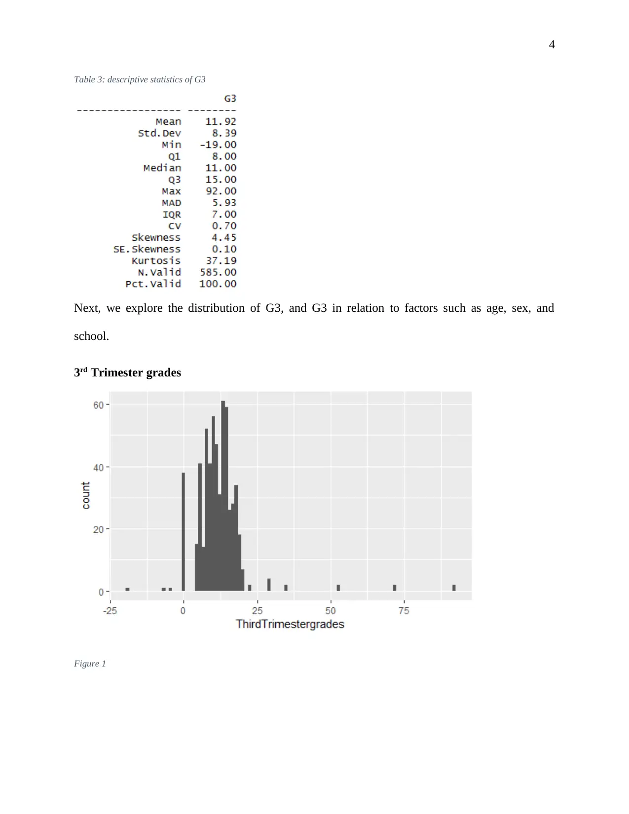
In table 3 below, we are presented with various descriptive statistics of the 3rd trimester grade
results.
⊘ This is a preview!⊘
Do you want full access?
Subscribe today to unlock all pages.

Trusted by 1+ million students worldwide
4
Table 3: descriptive statistics of G3
Next, we explore the distribution of G3, and G3 in relation to factors such as age, sex, and
school.
3rd Trimester grades
Figure 1
Table 3: descriptive statistics of G3
Next, we explore the distribution of G3, and G3 in relation to factors such as age, sex, and
school.
3rd Trimester grades
Figure 1
Paraphrase This Document
Need a fresh take? Get an instant paraphrase of this document with our AI Paraphraser
5
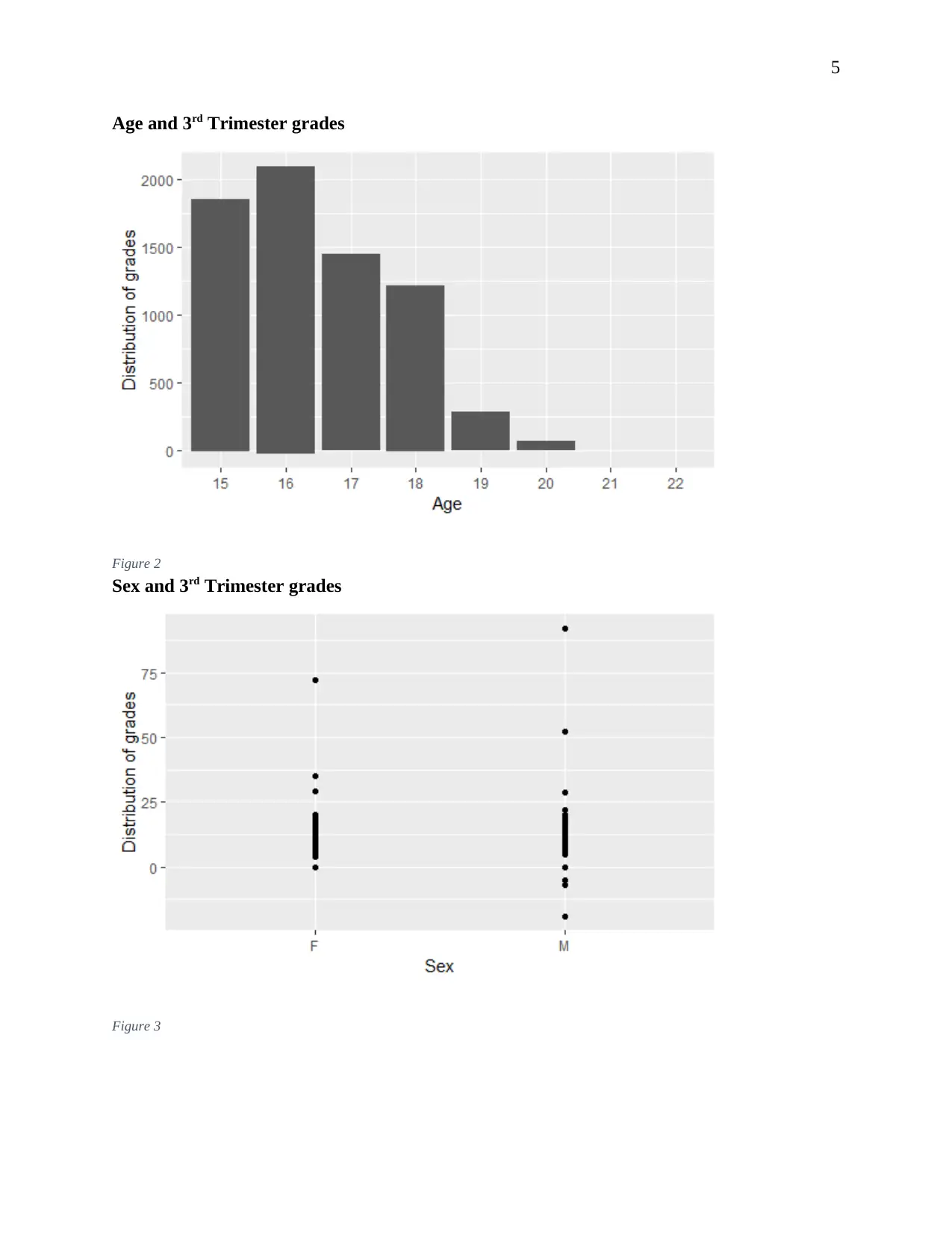
Age and 3rd Trimester grades
Figure 2
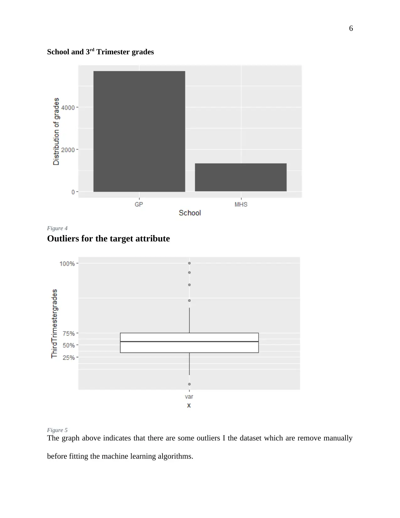
Sex and 3rd Trimester grades
Figure 3
Age and 3rd Trimester grades
Figure 2
Sex and 3rd Trimester grades
Figure 3
6
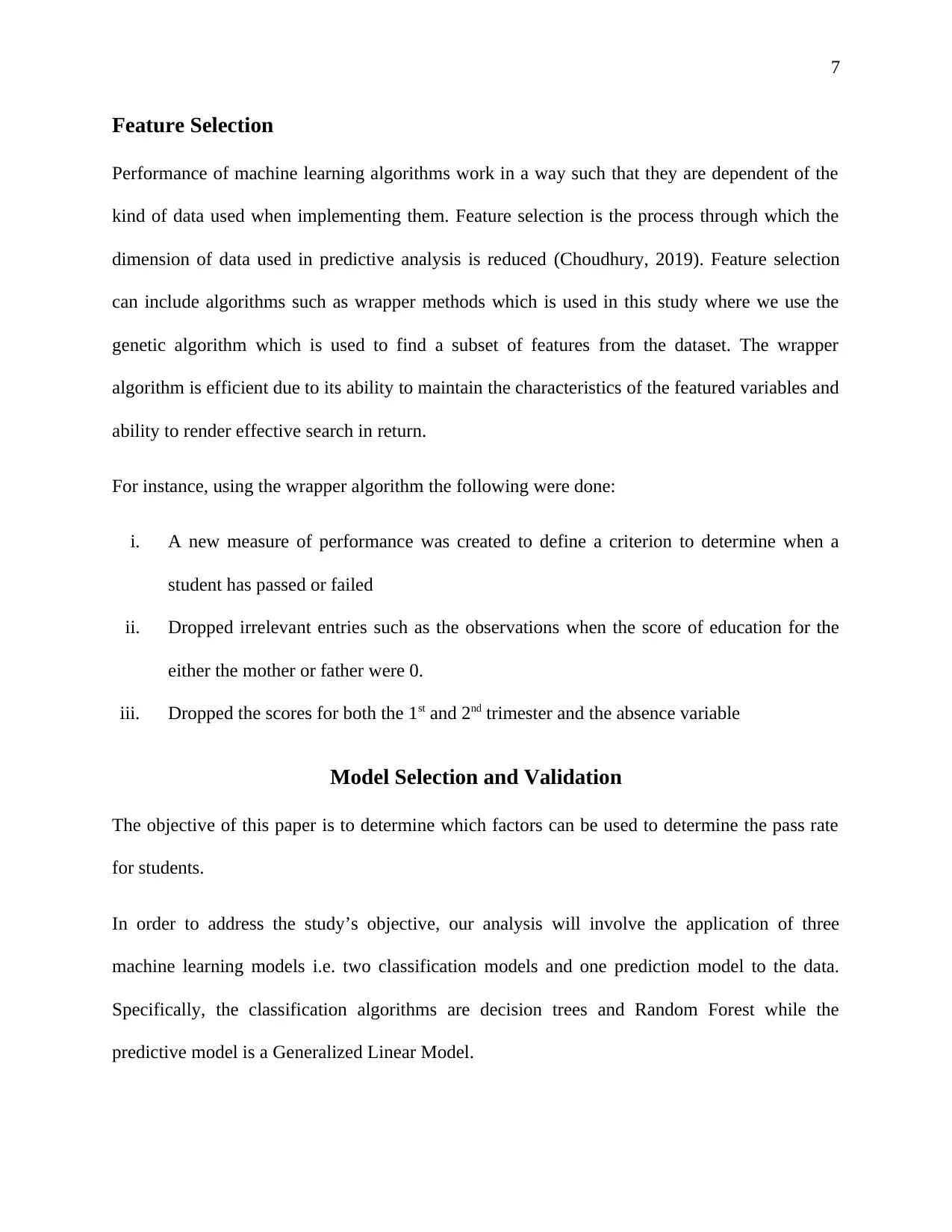
School and 3rd Trimester grades
Figure 4
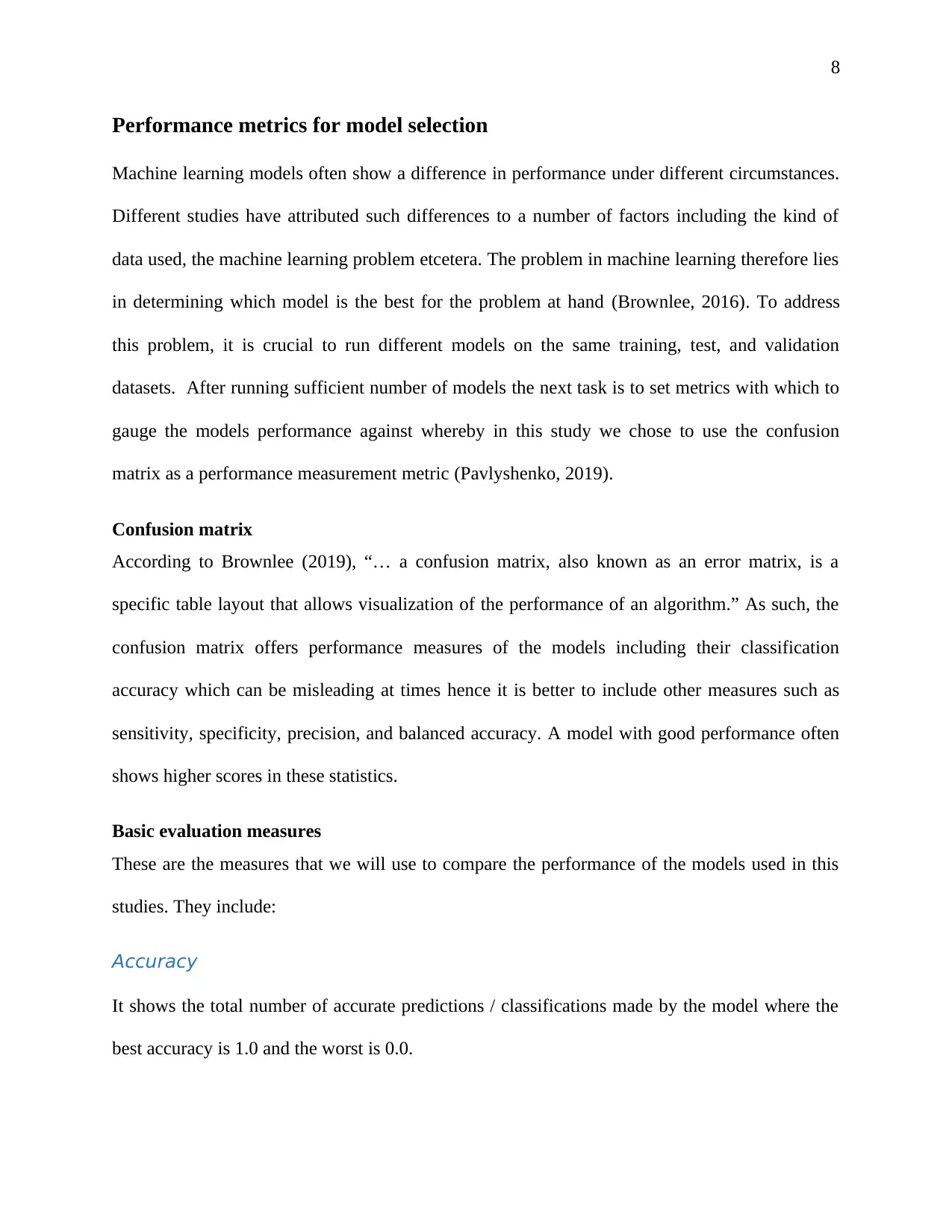
Outliers for the target attribute
Figure 5
The graph above indicates that there are some outliers I the dataset which are remove manually
before fitting the machine learning algorithms.
School and 3rd Trimester grades
Figure 4
Outliers for the target attribute
Figure 5
The graph above indicates that there are some outliers I the dataset which are remove manually
before fitting the machine learning algorithms.
⊘ This is a preview!⊘
Do you want full access?
Subscribe today to unlock all pages.

Trusted by 1+ million students worldwide
7
Feature Selection
Performance of machine learning algorithms work in a way such that they are dependent of the
kind of data used when implementing them. Feature selection is the process through which the
dimension of data used in predictive analysis is reduced (Choudhury, 2019). Feature selection
can include algorithms such as wrapper methods which is used in this study where we use the
genetic algorithm which is used to find a subset of features from the dataset. The wrapper
algorithm is efficient due to its ability to maintain the characteristics of the featured variables and
ability to render effective search in return.
For instance, using the wrapper algorithm the following were done:
i. A new measure of performance was created to define a criterion to determine when a
student has passed or failed
ii. Dropped irrelevant entries such as the observations when the score of education for the
either the mother or father were 0.
iii. Dropped the scores for both the 1st and 2nd trimester and the absence variable
Model Selection and Validation
The objective of this paper is to determine which factors can be used to determine the pass rate
for students.
In order to address the study’s objective, our analysis will involve the application of three
machine learning models i.e. two classification models and one prediction model to the data.
Specifically, the classification algorithms are decision trees and Random Forest while the
predictive model is a Generalized Linear Model.
Paraphrase This Document
Need a fresh take? Get an instant paraphrase of this document with our AI Paraphraser
8
Performance metrics for model selection
Machine learning models often show a difference in performance under different circumstances.
Different studies have attributed such differences to a number of factors including the kind of
data used, the machine learning problem etcetera. The problem in machine learning therefore lies
in determining which model is the best for the problem at hand (Brownlee, 2016). To address
this problem, it is crucial to run different models on the same training, test, and validation
datasets. After running sufficient number of models the next task is to set metrics with which to
gauge the models performance against whereby in this study we chose to use the confusion
matrix as a performance measurement metric (Pavlyshenko, 2019).
Confusion matrix
According to Brownlee (2019), “… a confusion matrix, also known as an error matrix, is a
specific table layout that allows visualization of the performance of an algorithm.” As such, the
confusion matrix offers performance measures of the models including their classification
accuracy which can be misleading at times hence it is better to include other measures such as
sensitivity, specificity, precision, and balanced accuracy. A model with good performance often
shows higher scores in these statistics.
Basic evaluation measures
These are the measures that we will use to compare the performance of the models used in this
studies. They include:
Accuracy
It shows the total number of accurate predictions / classifications made by the model where the
best accuracy is 1.0 and the worst is 0.0.
9
Prevalence and Precision
Prevalence is a measure of how often the positives (yes) occurs in the sample while precision is a
measure of how accurate the model predicts yeas in the sample
Sensitivity and specificity
While sensitivity measures the proportion of actual positives that are identified by the model,
specificity measures the true negatives that have been correctly identified by the model.
Generalized Linear Model (GLMs)
Unlike a linear model which assume that the outcome of input features into the model will have a
Gaussian distribution, GLMs assume that the outcomes are Non-Gaussian. In the linear models,
the prediction of categorical outcomes are restricted in which case a GLM is adopted as an
extension (Molnar, 2019). The basic idea for GLM build up is: “Keep the weighted sum of the
features, but allow non-Gaussian outcome distributions and connect the expected mean of this
distribution and the weighted sum through a possibly nonlinear function” (Molnar, 2019). GLM
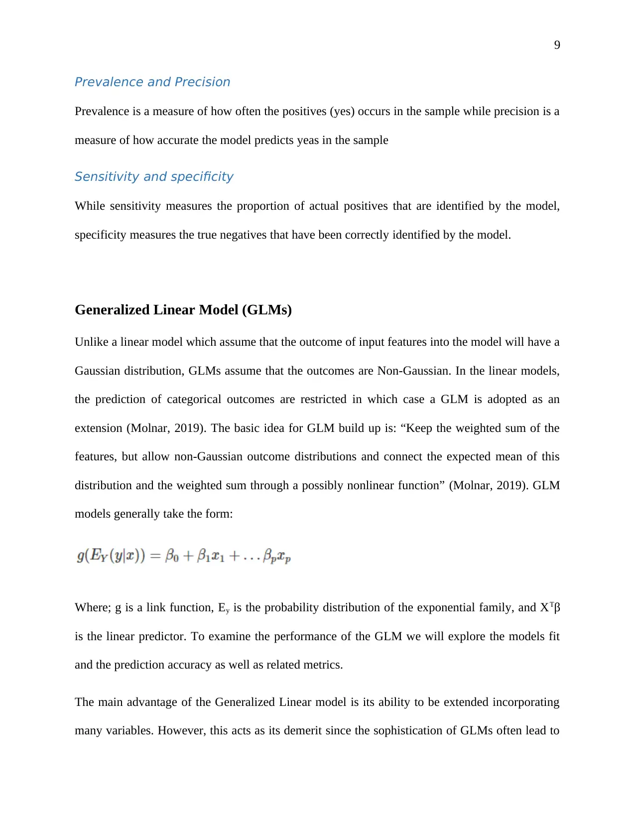
models generally take the form:
Where; g is a link function, Ey is the probability distribution of the exponential family, and XTβ
is the linear predictor. To examine the performance of the GLM we will explore the models fit
and the prediction accuracy as well as related metrics.
The main advantage of the Generalized Linear model is its ability to be extended incorporating
many variables. However, this acts as its demerit since the sophistication of GLMs often lead to
⊘ This is a preview!⊘
Do you want full access?
Subscribe today to unlock all pages.

Trusted by 1+ million students worldwide
10
problems in interpretation and at times fail to work in situations where there are non-linear
features (Molnar, 2019).
Implementation results
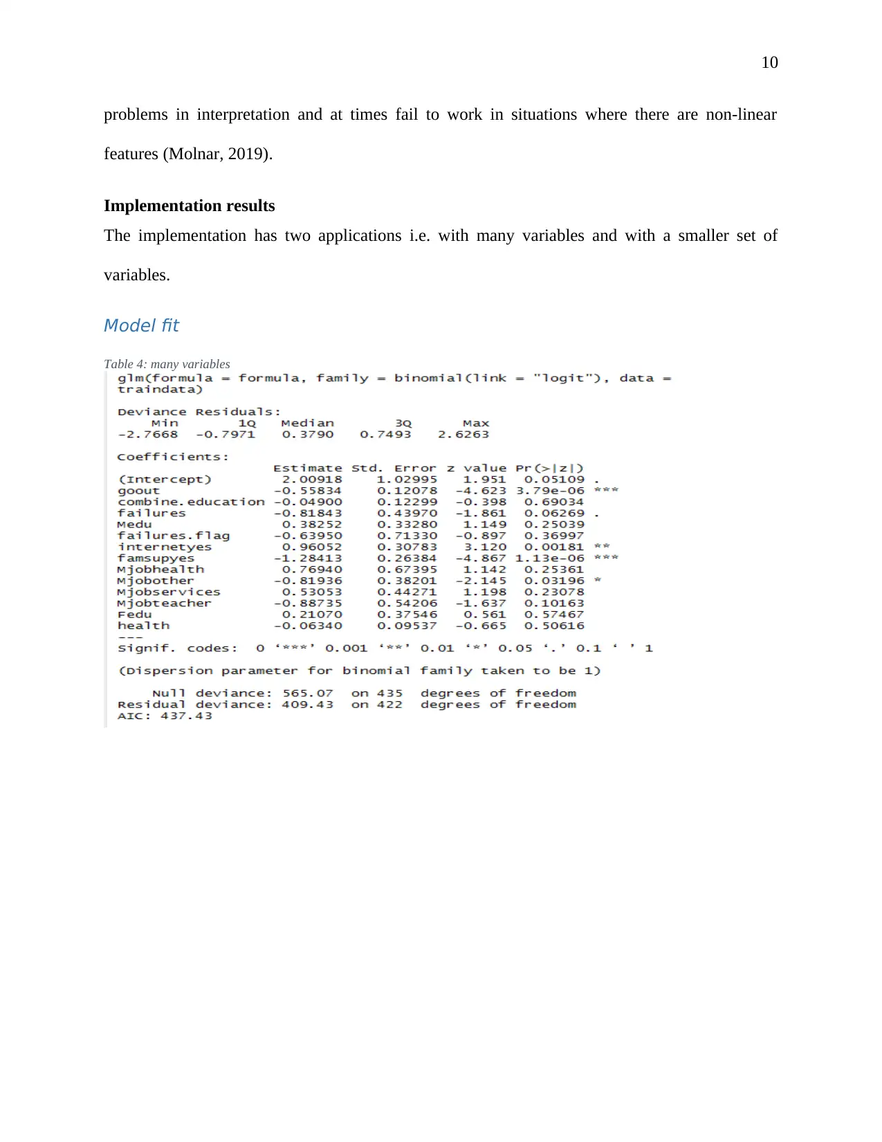
The implementation has two applications i.e. with many variables and with a smaller set of
variables.
Model fit
Table 4: many variables
problems in interpretation and at times fail to work in situations where there are non-linear
features (Molnar, 2019).
Implementation results
The implementation has two applications i.e. with many variables and with a smaller set of
variables.
Model fit
Table 4: many variables
Paraphrase This Document
Need a fresh take? Get an instant paraphrase of this document with our AI Paraphraser
11
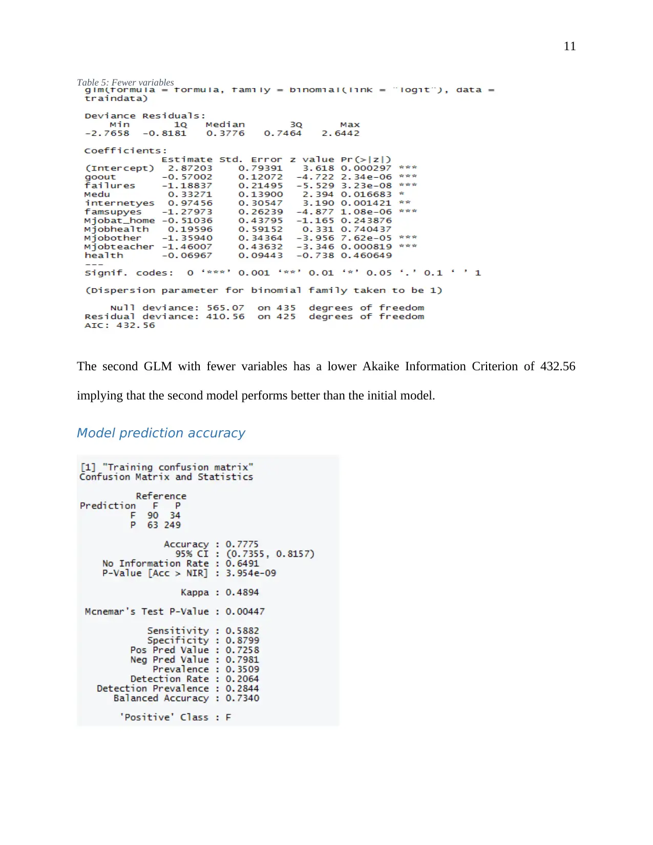
Table 5: Fewer variables
The second GLM with fewer variables has a lower Akaike Information Criterion of 432.56
implying that the second model performs better than the initial model.
Model prediction accuracy
Table 5: Fewer variables
The second GLM with fewer variables has a lower Akaike Information Criterion of 432.56
implying that the second model performs better than the initial model.
Model prediction accuracy
12
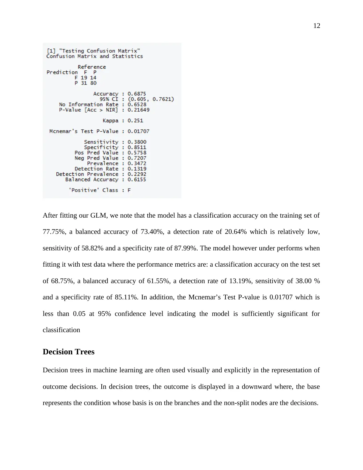
After fitting our GLM, we note that the model has a classification accuracy on the training set of
77.75%, a balanced accuracy of 73.40%, a detection rate of 20.64% which is relatively low,
sensitivity of 58.82% and a specificity rate of 87.99%. The model however under performs when
fitting it with test data where the performance metrics are: a classification accuracy on the test set
of 68.75%, a balanced accuracy of 61.55%, a detection rate of 13.19%, sensitivity of 38.00 %
and a specificity rate of 85.11%. In addition, the Mcnemar’s Test P-value is 0.01707 which is
less than 0.05 at 95% confidence level indicating the model is sufficiently significant for
classification
Decision Trees
Decision trees in machine learning are often used visually and explicitly in the representation of
outcome decisions. In decision trees, the outcome is displayed in a downward where, the base
represents the condition whose basis is on the branches and the non-split nodes are the decisions.
⊘ This is a preview!⊘
Do you want full access?
Subscribe today to unlock all pages.

Trusted by 1+ million students worldwide
1 out of 23
Related Documents
Your All-in-One AI-Powered Toolkit for Academic Success.
+13062052269
info@desklib.com
Available 24*7 on WhatsApp / Email
![[object Object]](/_next/static/media/star-bottom.7253800d.svg)
Unlock your academic potential
Copyright © 2020–2026 A2Z Services. All Rights Reserved. Developed and managed by ZUCOL.


