Macquarie University ECON334: Financial Econometrics Assignment

This financial econometrics assignment focuses on time series analysis and forecasting, utilizing the 'SPREAD' dataset from 1957M01 to 2015M03. The assignment involves plotting the data, calculating Autocorrelation (ACF) and Partial Autocorrelation Functions (PACF), and selecting the best ARIMA model based on the Akaike Information Criterion (AIC). The analysis compares static and rolling window forecasting methods, as well as one-step-ahead and dynamic forecasting. The assignment also includes forecast evaluation, and considers the Ljung-Box test for residuals, using the chi-square test to assess autocorrelation. The results from different AR models are presented, along with forecast evaluation statistics such as RMSE, MAE, MAPE, SMAPE, Theil U1, and Theil U2. The concluding remarks discuss the trends and accuracy of the forecasting models applied to the 'SPREAD' data.

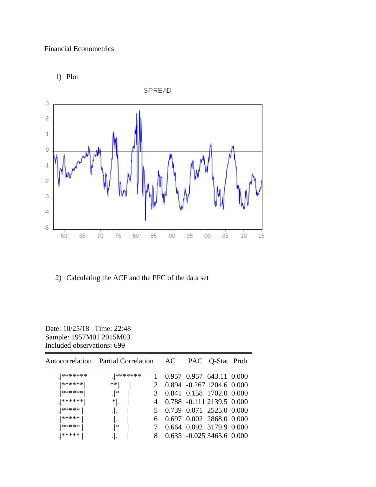
Financial Econometrics
1) Plot
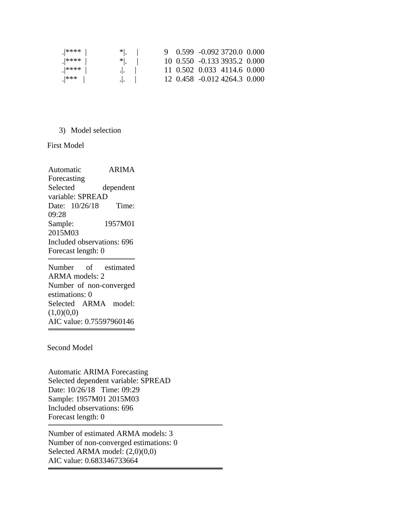
2) Calculating the ACF and the PFC of the data set
Date: 10/25/18 Time: 22:48
Sample: 1957M01 2015M03
Included observations: 699
Autocorrelation Partial Correlation AC PAC Q-Stat Prob
.|******* .|******* 1 0.957 0.957 643.11 0.000
.|******| **|. | 2 0.894 -0.267 1204.6 0.000
.|******| .|* | 3 0.841 0.158 1702.0 0.000
.|******| *|. | 4 0.788 -0.111 2139.5 0.000
.|***** | .|. | 5 0.739 0.071 2525.0 0.000
.|***** | .|. | 6 0.697 0.002 2868.0 0.000
.|***** | .|* | 7 0.664 0.092 3179.9 0.000
.|***** | .|. | 8 0.635 -0.025 3465.6 0.000

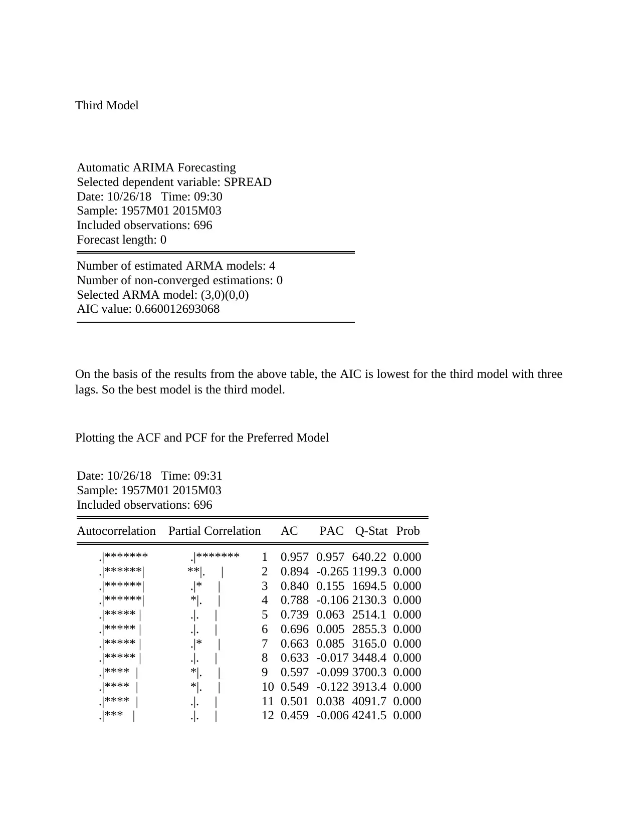
.|**** | *|. | 9 0.599 -0.092 3720.0 0.000
.|**** | *|. | 10 0.550 -0.133 3935.2 0.000
.|**** | .|. | 11 0.502 0.033 4114.6 0.000
.|*** | .|. | 12 0.458 -0.012 4264.3 0.000
3) Model selection
First Model
Automatic ARIMA
Forecasting
Selected dependent
variable: SPREAD
Date: 10/26/18 Time:
09:28
Sample: 1957M01
2015M03
Included observations: 696
Forecast length: 0
Number of estimated
ARMA models: 2
Number of non-converged
estimations: 0
Selected ARMA model:
(1,0)(0,0)
AIC value: 0.75597960146
Second Model
Automatic ARIMA Forecasting
Selected dependent variable: SPREAD
Date: 10/26/18 Time: 09:29
Sample: 1957M01 2015M03
Included observations: 696
Forecast length: 0
Number of estimated ARMA models: 3
Number of non-converged estimations: 0
Selected ARMA model: (2,0)(0,0)
AIC value: 0.683346733664

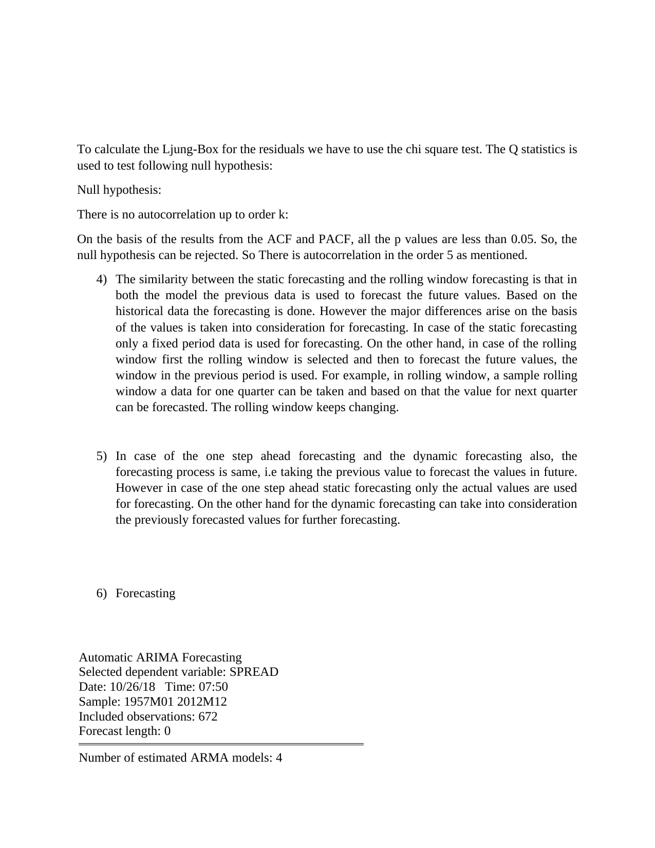
Third Model
Automatic ARIMA Forecasting
Selected dependent variable: SPREAD
Date: 10/26/18 Time: 09:30
Sample: 1957M01 2015M03
Included observations: 696
Forecast length: 0
Number of estimated ARMA models: 4
Number of non-converged estimations: 0
Selected ARMA model: (3,0)(0,0)
AIC value: 0.660012693068
On the basis of the results from the above table, the AIC is lowest for the third model with three
lags. So the best model is the third model.
Plotting the ACF and PCF for the Preferred Model
Date: 10/26/18 Time: 09:31
Sample: 1957M01 2015M03
Included observations: 696
Autocorrelation Partial Correlation AC PAC Q-Stat Prob
.|******* .|******* 1 0.957 0.957 640.22 0.000
.|******| **|. | 2 0.894 -0.265 1199.3 0.000
.|******| .|* | 3 0.840 0.155 1694.5 0.000
.|******| *|. | 4 0.788 -0.106 2130.3 0.000
.|***** | .|. | 5 0.739 0.063 2514.1 0.000
.|***** | .|. | 6 0.696 0.005 2855.3 0.000
.|***** | .|* | 7 0.663 0.085 3165.0 0.000
.|***** | .|. | 8 0.633 -0.017 3448.4 0.000
.|**** | *|. | 9 0.597 -0.099 3700.3 0.000
.|**** | *|. | 10 0.549 -0.122 3913.4 0.000
.|**** | .|. | 11 0.501 0.038 4091.7 0.000
.|*** | .|. | 12 0.459 -0.006 4241.5 0.000

To calculate the Ljung-Box for the residuals we have to use the chi square test. The Q statistics is
used to test following null hypothesis:
Null hypothesis:
There is no autocorrelation up to order k:
On the basis of the results from the ACF and PACF, all the p values are less than 0.05. So, the
null hypothesis can be rejected. So There is autocorrelation in the order 5 as mentioned.
4) The similarity between the static forecasting and the rolling window forecasting is that in
both the model the previous data is used to forecast the future values. Based on the
historical data the forecasting is done. However the major differences arise on the basis
of the values is taken into consideration for forecasting. In case of the static forecasting
only a fixed period data is used for forecasting. On the other hand, in case of the rolling
window first the rolling window is selected and then to forecast the future values, the
window in the previous period is used. For example, in rolling window, a sample rolling
window a data for one quarter can be taken and based on that the value for next quarter
can be forecasted. The rolling window keeps changing.
5) In case of the one step ahead forecasting and the dynamic forecasting also, the
forecasting process is same, i.e taking the previous value to forecast the values in future.
However in case of the one step ahead static forecasting only the actual values are used
for forecasting. On the other hand for the dynamic forecasting can take into consideration
the previously forecasted values for further forecasting.
6) Forecasting
Automatic ARIMA Forecasting
Selected dependent variable: SPREAD
Date: 10/26/18 Time: 07:50
Sample: 1957M01 2012M12
Included observations: 672
Forecast length: 0
Number of estimated ARMA models: 4

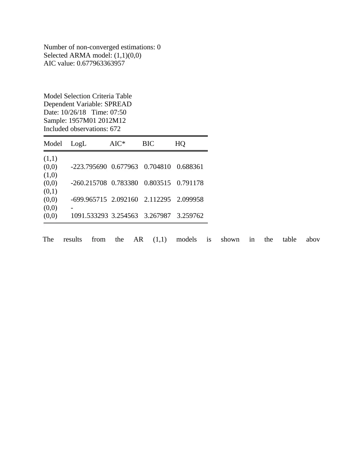
Number of non-converged estimations: 0
Selected ARMA model: (1,1)(0,0)
AIC value: 0.677963363957
Model Selection Criteria Table
Dependent Variable: SPREAD
Date: 10/26/18 Time: 07:50
Sample: 1957M01 2012M12
Included observations: 672
Model LogL AIC* BIC HQ
(1,1)
(0,0) -223.795690 0.677963 0.704810 0.688361
(1,0)
(0,0) -260.215708 0.783380 0.803515 0.791178
(0,1)
(0,0) -699.965715 2.092160 2.112295 2.099958
(0,0)
(0,0)
-
1091.533293 3.254563 3.267987 3.259762
The results from the AR (1,1) models is shown in the table abov

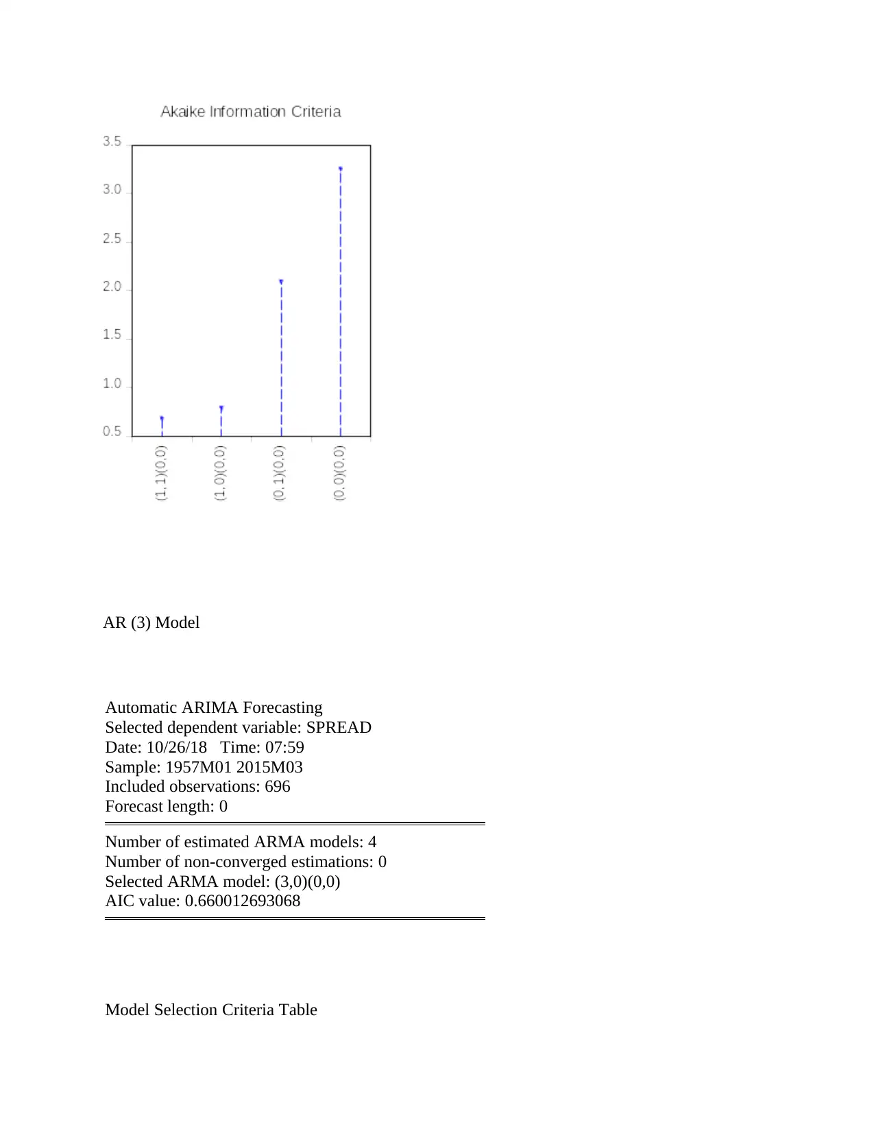
AR (3) Model
Automatic ARIMA Forecasting
Selected dependent variable: SPREAD
Date: 10/26/18 Time: 07:59
Sample: 1957M01 2015M03
Included observations: 696
Forecast length: 0
Number of estimated ARMA models: 4
Number of non-converged estimations: 0
Selected ARMA model: (3,0)(0,0)
AIC value: 0.660012693068
Model Selection Criteria Table

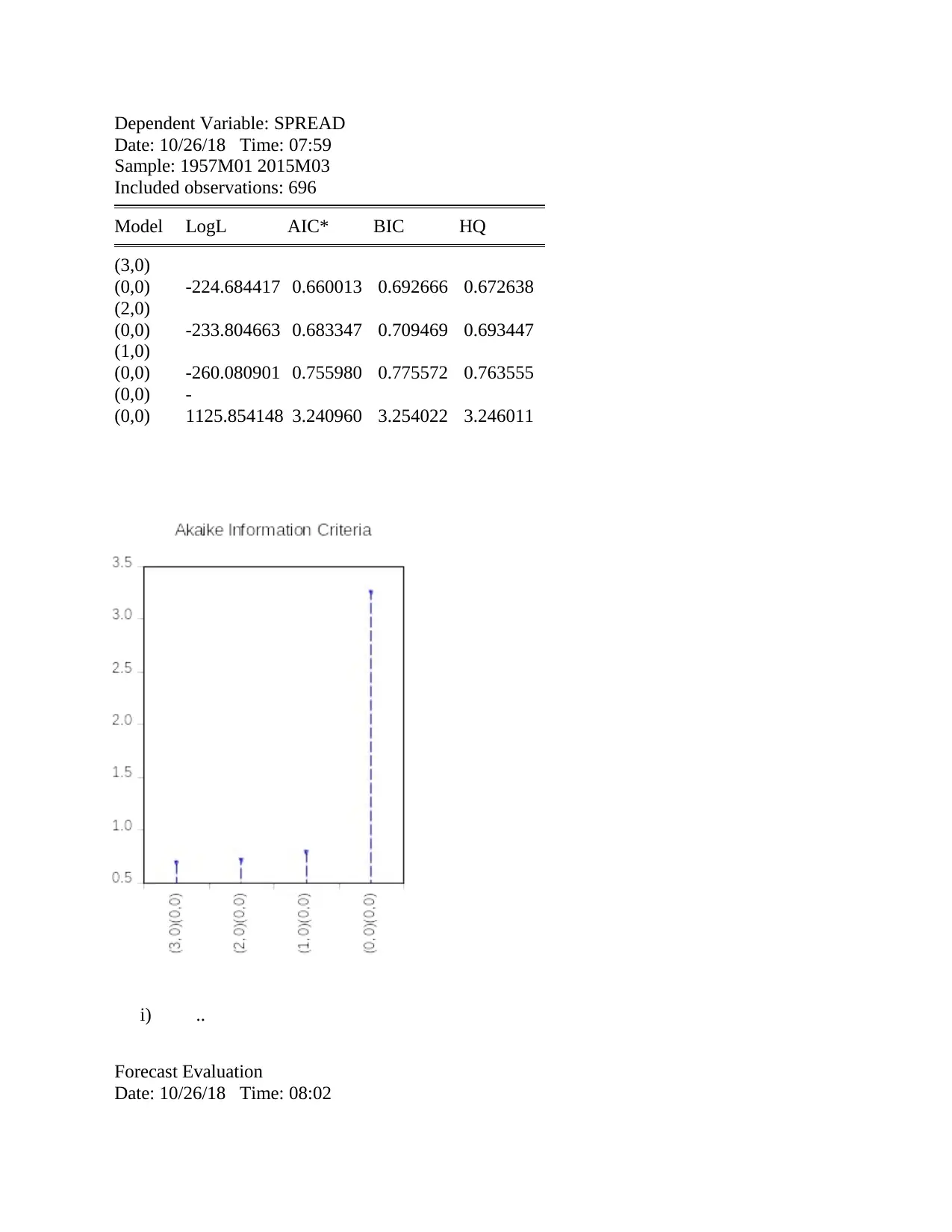
Dependent Variable: SPREAD
Date: 10/26/18 Time: 07:59
Sample: 1957M01 2015M03
Included observations: 696
Model LogL AIC* BIC HQ
(3,0)
(0,0) -224.684417 0.660013 0.692666 0.672638
(2,0)
(0,0) -233.804663 0.683347 0.709469 0.693447
(1,0)
(0,0) -260.080901 0.755980 0.775572 0.763555
(0,0)
(0,0)
-
1125.854148 3.240960 3.254022 3.246011
i) ..
Forecast Evaluation
Date: 10/26/18 Time: 08:02

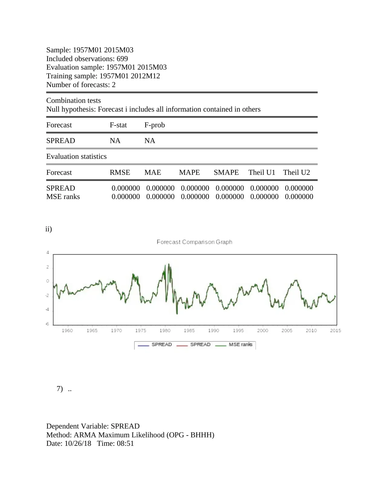
Sample: 1957M01 2015M03
Included observations: 699
Evaluation sample: 1957M01 2015M03
Training sample: 1957M01 2012M12
Number of forecasts: 2
Combination tests
Null hypothesis: Forecast i includes all information contained in others
Forecast F-stat F-prob
SPREAD NA NA
Evaluation statistics
Forecast RMSE MAE MAPE SMAPE Theil U1 Theil U2
SPREAD 0.000000 0.000000 0.000000 0.000000 0.000000 0.000000
MSE ranks 0.000000 0.000000 0.000000 0.000000 0.000000 0.000000
ii)
7) ..
Dependent Variable: SPREAD
Method: ARMA Maximum Likelihood (OPG - BHHH)
Date: 10/26/18 Time: 08:51

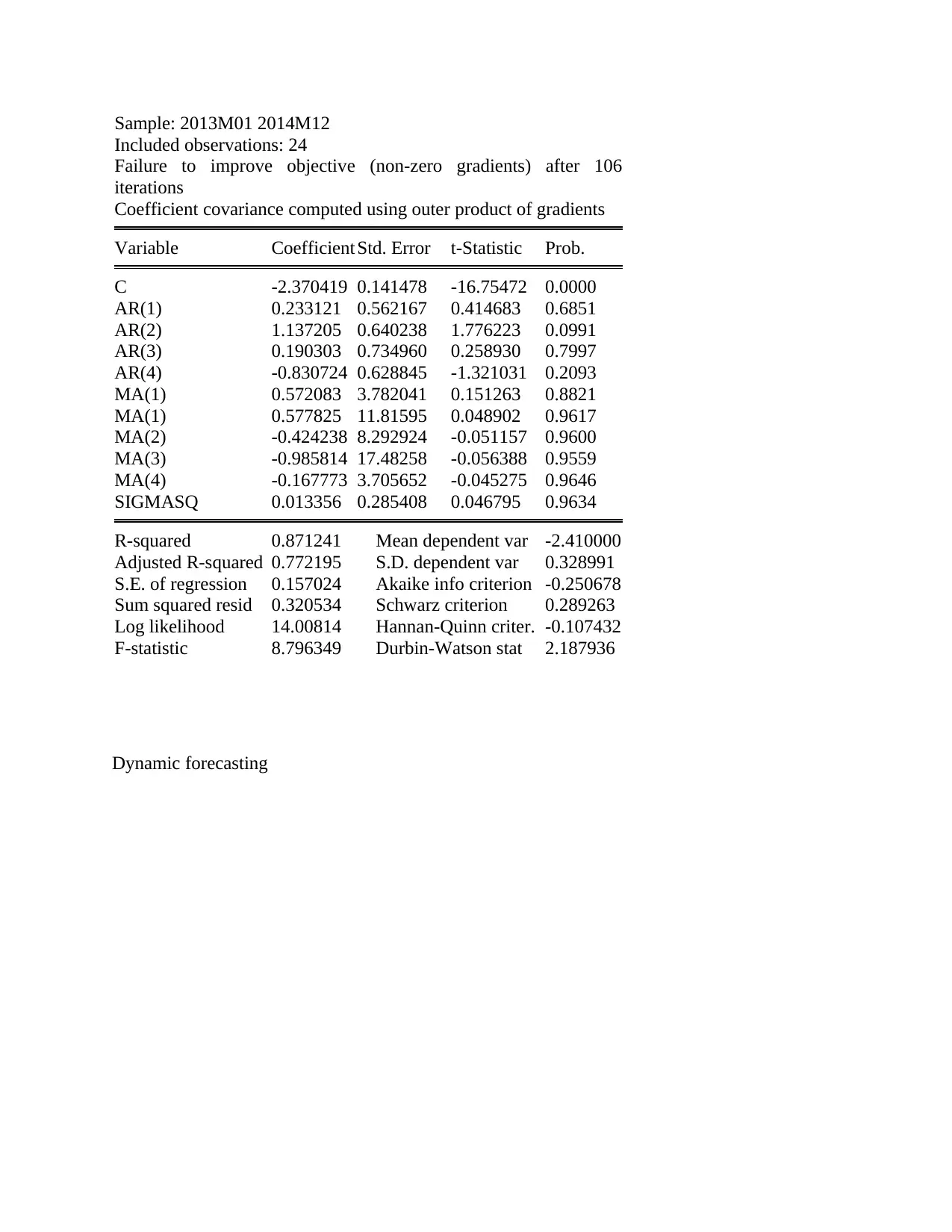
Sample: 2013M01 2014M12
Included observations: 24
Failure to improve objective (non-zero gradients) after 106
iterations
Coefficient covariance computed using outer product of gradients
Variable Coefficient Std. Error t-Statistic Prob.
C -2.370419 0.141478 -16.75472 0.0000
AR(1) 0.233121 0.562167 0.414683 0.6851
AR(2) 1.137205 0.640238 1.776223 0.0991
AR(3) 0.190303 0.734960 0.258930 0.7997
AR(4) -0.830724 0.628845 -1.321031 0.2093
MA(1) 0.572083 3.782041 0.151263 0.8821
MA(1) 0.577825 11.81595 0.048902 0.9617
MA(2) -0.424238 8.292924 -0.051157 0.9600
MA(3) -0.985814 17.48258 -0.056388 0.9559
MA(4) -0.167773 3.705652 -0.045275 0.9646
SIGMASQ 0.013356 0.285408 0.046795 0.9634
R-squared 0.871241 Mean dependent var -2.410000
Adjusted R-squared 0.772195 S.D. dependent var 0.328991
S.E. of regression 0.157024 Akaike info criterion -0.250678
Sum squared resid 0.320534 Schwarz criterion 0.289263
Log likelihood 14.00814 Hannan-Quinn criter. -0.107432
F-statistic 8.796349 Durbin-Watson stat 2.187936
Dynamic forecasting

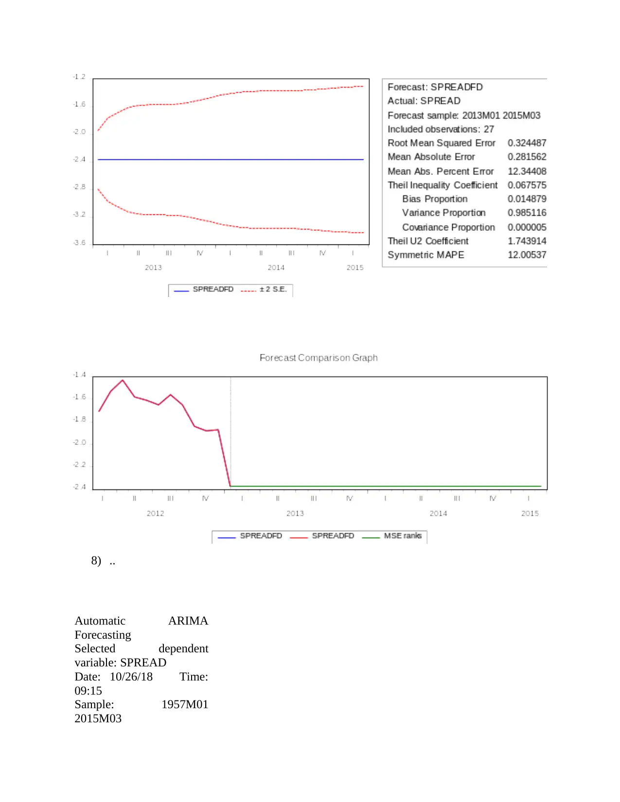
8) ..
Automatic ARIMA
Forecasting
Selected dependent
variable: SPREAD
Date: 10/26/18 Time:
09:15
Sample: 1957M01
2015M03

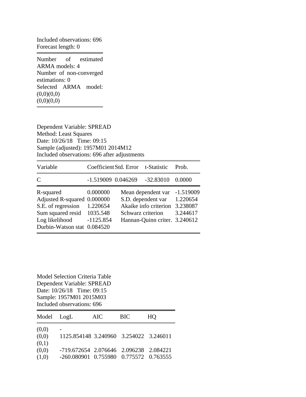
Included observations: 696
Forecast length: 0
Number of estimated
ARMA models: 4
Number of non-converged
estimations: 0
Selected ARMA model:
(0,0)(0,0)
(0,0)(0,0)
Dependent Variable: SPREAD
Method: Least Squares
Date: 10/26/18 Time: 09:15
Sample (adjusted): 1957M01 2014M12
Included observations: 696 after adjustments
Variable Coefficient Std. Error t-Statistic Prob.
C -1.519009 0.046269 -32.83010 0.0000
R-squared 0.000000 Mean dependent var -1.519009
Adjusted R-squared 0.000000 S.D. dependent var 1.220654
S.E. of regression 1.220654 Akaike info criterion 3.238087
Sum squared resid 1035.548 Schwarz criterion 3.244617
Log likelihood -1125.854 Hannan-Quinn criter. 3.240612
Durbin-Watson stat 0.084520
Model Selection Criteria Table
Dependent Variable: SPREAD
Date: 10/26/18 Time: 09:15
Sample: 1957M01 2015M03
Included observations: 696
Model LogL AIC BIC HQ
(0,0)
(0,0)
-
1125.854148 3.240960 3.254022 3.246011
(0,1)
(0,0) -719.672654 2.076646 2.096238 2.084221
(1,0) -260.080901 0.755980 0.775572 0.763555

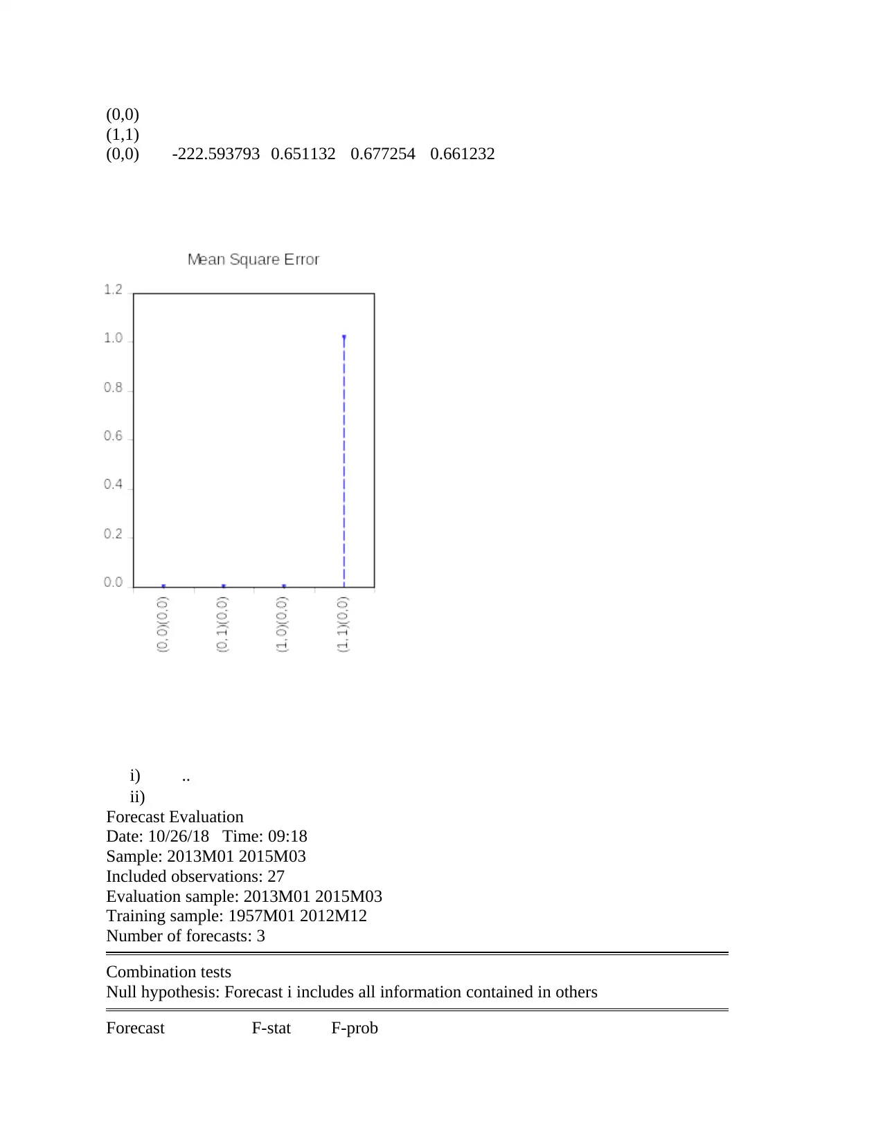
(0,0)
(1,1)
(0,0) -222.593793 0.651132 0.677254 0.661232
i) ..
ii)
Forecast Evaluation
Date: 10/26/18 Time: 09:18
Sample: 2013M01 2015M03
Included observations: 27
Evaluation sample: 2013M01 2015M03
Training sample: 1957M01 2012M12
Number of forecasts: 3
Combination tests
Null hypothesis: Forecast i includes all information contained in others
Forecast F-stat F-prob