Macroeconomics Assignment: Economic Models and Policy Analysis

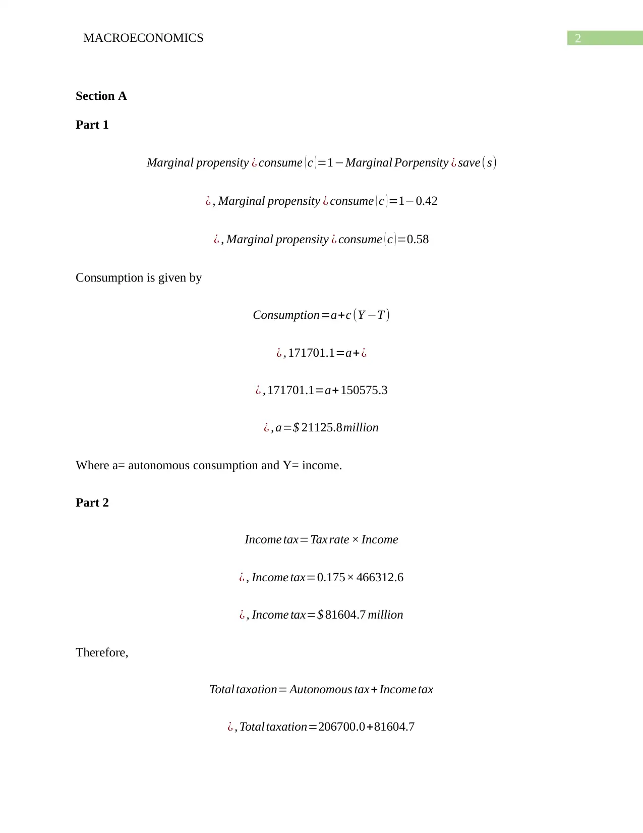
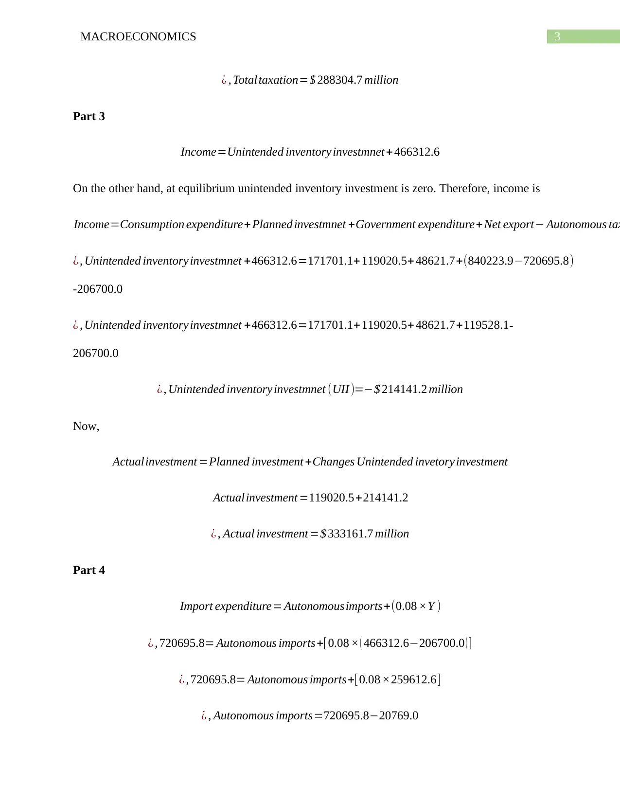
This macroeconomics assignment analyzes an economic scenario, covering various aspects of macroeconomic principles. It begins with consumption function and equilibrium income calculations, followed by an analysis of aggregate expenditure (AE) and aggregate demand-aggregate supply (AD-AS) models. The assignment explores the impact of unplanned inventory investment, the effects of fiscal policy, and the role of monetary policy in closing a GDP gap. It also examines the exchange rate market, illustrating the effects of interest rate changes and their implications on exports, employment, and overall economic expansion. The solution includes calculations, graphical representations, and explanations of economic concepts, referencing relevant academic literature to support the analysis.

Running head: MACROECONOMICS
Macroeconomics
Name of the Student
Name of the University
Student ID

1MACROECONOMICS
Table of Contents
Section A.........................................................................................................................................2
Section B..........................................................................................................................................7
Reference.......................................................................................................................................13

2MACROECONOMICS
Section A
Part 1
Marginal propensity ¿ consume ( c ) =1−Marginal Porpensity ¿ save (s)
¿ , Marginal propensity ¿ consume ( c )=1−0.42
¿ , Marginal propensity ¿ consume ( c ) =0.58
Consumption is given by
Consumption=a+c (Y −T )
¿ , 171701.1=a+¿
¿ , 171701.1=a+ 150575.3
¿ , a=$ 21125.8million
Where a= autonomous consumption and Y= income.
Part 2
Income tax=Taxrate × Income
¿ , Income tax=0.175× 466312.6
¿ , Income tax=$ 81604.7 million
Therefore,
Total taxation= Autonomous tax+ Income tax
¿ , Total taxation=206700.0+81604.7

3MACROECONOMICS
¿ , Totaltaxation=$ 288304.7 million
Part 3
Income=Unintended inventory investmnet + 466312.6
On the other hand, at equilibrium unintended inventory investment is zero. Therefore, income is
Income=Consumption expenditure+ Planned investmnet +Government expenditure+ Net export− Autonomous tax
¿ , Unintended inventory investmnet +466312.6=171701.1+ 119020.5+ 48621.7+(840223.9−720695.8)
-206700.0
¿ , Unintended inventory investmnet +466312.6=171701.1+119020.5+48621.7+119528.1-
206700.0
¿ , Unintended inventory investmnet (UII )=−$ 214141.2 million
Now,
Actualinvestment =Planned investment +Changes Unintended invetory investment
Actualinvestment =119020.5+214141.2
¿ , Actual investment =$ 333161.7 million
Part 4
Import expenditure= Autonomousimports+(0.08 ×Y )
¿ , 720695.8= Autonomous imports+[0.08 × ( 466312.6−206700.0 ) ]
¿ , 720695.8= Autonomous imports+[0.08 ×259612.6]
¿ , Autonomous imports=720695.8−20769.0

4MACROECONOMICS
¿ , Autonomous imports=$ 699926.8million
Part 5
Marginal propensity ¿ export=1−Marginal propensity ¿ import
¿ , Marginal propensity ¿ export=1−0.08
¿ , Marginal propensity ¿ export=0.92
Now,
Export expenditure= Autonomous exports+(0.92× 259612.6)
¿ , Autonomous exports=840223.9−238843.6
¿ , Autonomous exports=$ 601380.3 million
Therefore,
Autonomous net exports=Autonomous exports− Autonomous imports
¿ , Autonomous net exports=601380.3−699926.8
¿ , Autonomous net exports=$−98546.5 million
Part 6
Autonomous planned expenditure=Autonomous consumption+ Autonomous investmnet +Governmnet expenditure
¿ , Autonomous planned expenditure=21125.8+9983.2+48621.7−206700.0
¿ , Autonomous planned expenditure=−$ 126969.3million
Part 7

5MACROECONOMICS
At income level of $466312.6million the economy is not in equilibrium since there is
existence unintended inventory investment. The equilibrium level of income is
Equilibrium income level=466312.6−214141.2
¿ , Equilibrium income level=$ 252171.4 million
Part 8
Figure 1: Aggregate
expenditure
Source: (Created by the Author)
It is evident from Figure 1 that the current equilibrium income is lower than actual level
of income. The unplanned inventory investment has boosting effect on the economy1. Due to this
investment, the production of the economy will rise along with employment and the disposable
1 Grasselli, M, & A Nguyen-Huu, "Inventory growth cycles with debt-financed investment.".
in Structural Change and Economic Dynamics, 44, 2018, 1-13.

6MACROECONOMICS
income. Consequently, the consumption demand will increase and thereby increases the
aggregate demand. With rise in aggregate demand the price level will rise2. Owing to increased
chance of profitability the aggregate supply further increases by the amount of rise is aggregate
demand. As a result, the income of the economy rises and reaches actual level. (100 words)
Part 9
Expenditure multiplier= 1
MPS
¿ , Expenditure multiplier = 1
0.42
¿ , Expenditure multiplier =2.4
Again,
Tax multiplier= MPC
MPS
¿ , Tax multiplier= 0.58
0.42
¿ , Tax multiplier=1.4
Section B
Part 10
GDP gap=450000.0−252171.4
2 Leduc, S, & Z Liu, "Uncertainty shocks are aggregate demand shocks.". in Journal of Monetary
Economics, 82, 2016, 20-35.

7MACROECONOMICS
¿ , GDP gap=$ 197828.6 million
Figure 2: AD- AS model
Source: (Created by the Author)
Figure 3: AE model

8MACROECONOMICS
Source: (Created by the Author)
Part 11
Change in spending required to close the existing gap is
Change∈spending=197828.6
2.4
Change∈spending=$ 82428.6 million
Part 12
288304.7−197828.6= Autonomous taxation+(0.175 ×450000.0)
¿ , 90476.1= Autonomous taxation+78750.0
¿ , Autonomous taxation=$ 11726.1 million
Therefore,
Change∈ Autonomous taxation=11726.1−206700.0
¿ , Change∈ Autonomous taxation=−$ 194973.9 million
Therefore, it is found that to close the gap the autonomous taxation need to decrease by -
$194973.9million.
Part 13

9MACROECONOMICS
The central bank of the country has decided to close the existing GDP gap but unwilling
to use fiscal policy. To close the GDP gap, the economy needs a boost and that can be caused by
increasing money supply. Therefore, the central bank uses expansionary monetary policy the by
lowering interest rate3. Subsequently, with fall in interest rate the amount of investment in the
economy increases because borrowing has become cheaper. On the other hand, under open
market operation the central bank buys back the bonds from market and thus the money supply
in the economy increases and boosts income.
Part 14
Figure 4: Exchange
rate market
Source: (Created by the Author)
3 Ndou, E, & T Mokoena, "How Does Inflation Impact the Effects of Expansionary Monetary Policy and
Fiscal Policies on Real GDP Growth?.". in Inequality, Output-Inflation Trade-Off and Economic Policy
Uncertainty, , 2019, 389-398.

10MACROECONOMICS
Fall in interest rate reduces the return on deposit and thus holding money is less
beneficial than previous scenario4. Owing to this, the foreign investors are less interested to hold
dollar and withdraw their investment from the economy. Following this, the demand for dollar
decreases and due to that the dollar demand curve moved inward to D1 from D. Given the
condition the supply of dollar in the economy rises and the supply curve moved to S1 from S.
Owing to this the supply of dollar in exchange rate market remains the same with lower
exchange rate at E*. (99 words)
Part 15
Figure 5: Impact on
economy and unemployment
Source: (Created by the Author)
4 Engel, C, "Exchange Rates, Interest Rates, and the Risk Premium.". in American Economic
Review, 106, 2016, 436-474.

11MACROECONOMICS
The fall in exchange rate of dollar means that value of dollar has depreciated in the
foreign exchange market5. Owing to that, the export goods become cheaper and thus the export
market will expand as foreign countries will increase their consumption of domestic good. With
expansion in the export sector there will be more employment causing the unemployment rate to
fall. Increase in employment and rise sales of export goods the income of the country increases6.
As a result, the economy of the country will expand. It is evident from figure 5 that output of the
economy has increased from Y to Y1.
5 Wang, F, Z Yin, & J Gan, "Exchange-rate fluctuation and pricing behavior in China’s wood-
based panel exporters: evidence from panel data.". in Canadian Journal of Forest Research, 47,
2017, 1392-1404.
6 Christiano, L, M Eichenbaum, & M Trabandt, "Unemployment and Business Cycles.".
in Econometrica, 84, 2016, 1523-1569.

12MACROECONOMICS
Reference
Christiano, L, M Eichenbaum, & M Trabandt, "Unemployment and Business Cycles.".
in Econometrica, 84, 2016, 1523-1569.
Engel, C, "Exchange Rates, Interest Rates, and the Risk Premium.". in American Economic
Review, 106, 2016, 436-474.
Grasselli, M, & A Nguyen-Huu, "Inventory growth cycles with debt-financed investment.".
in Structural Change and Economic Dynamics, 44, 2018, 1-13.
Leduc, S, & Z Liu, "Uncertainty shocks are aggregate demand shocks.". in Journal of Monetary
Economics, 82, 2016, 20-35.
Ndou, E, & T Mokoena, "How Does Inflation Impact the Effects of Expansionary Monetary
Policy and Fiscal Policies on Real GDP Growth?.". in Inequality, Output-Inflation Trade-Off and
Economic Policy Uncertainty, , 2019, 389-398.
Wang, F, Z Yin, & J Gan, "Exchange-rate fluctuation and pricing behavior in China’s wood-
based panel exporters: evidence from panel data.". in Canadian Journal of Forest Research, 47,
2017, 1392-1404.