Macroeconomics Assignment: Consumption, Investment, and Fiscal Policy

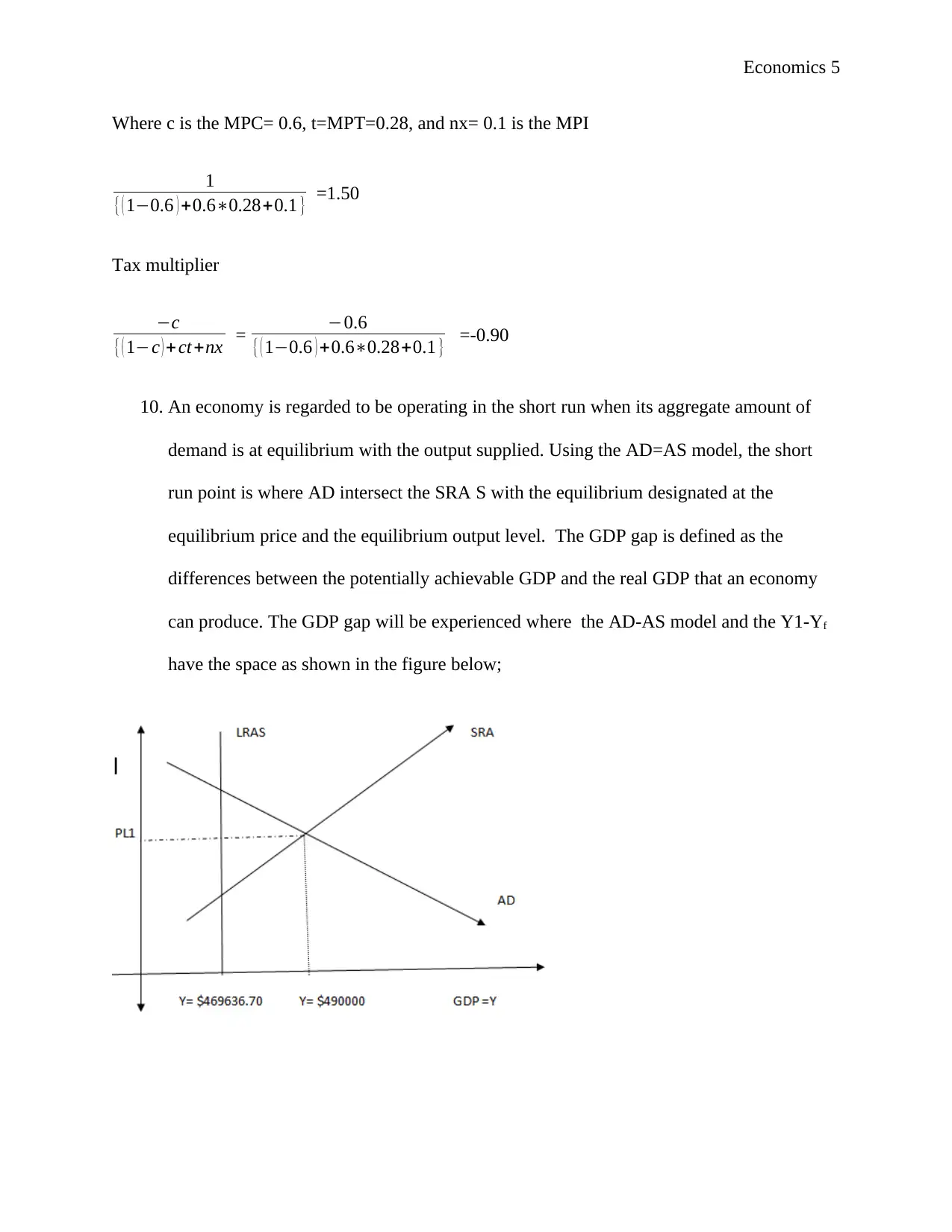
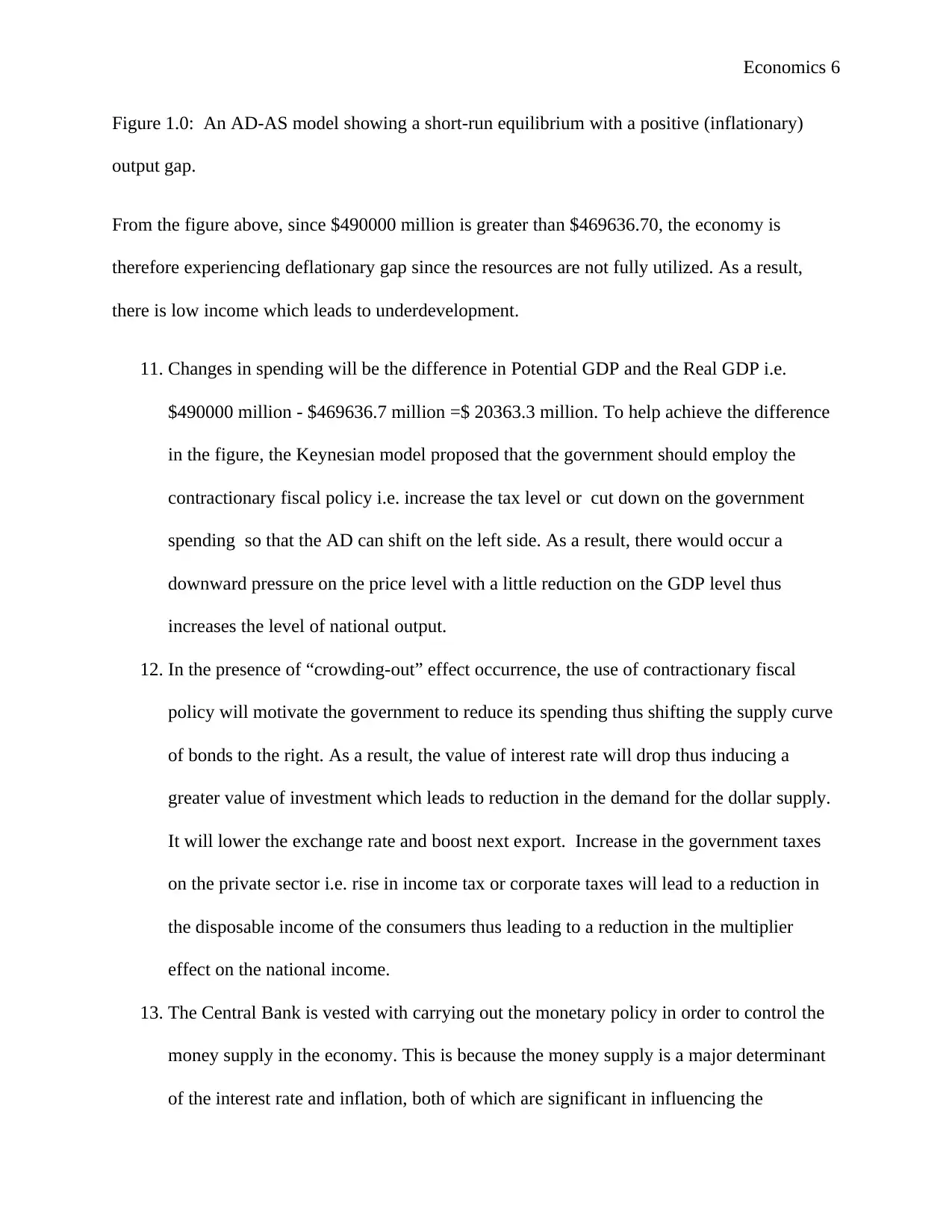
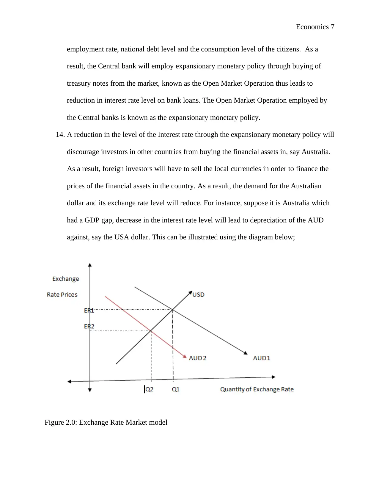
This macroeconomics assignment solution delves into various aspects of macroeconomic principles. It begins by calculating consumption expenditure, autonomous consumption, savings, and investment based on given data. It then explores import expenditure, autonomous net exports, and planned expenditure. The solution determines the equilibrium level, marginal leakage rate, and calculates expenditure and tax multipliers. The assignment also analyzes the short-run equilibrium using the AD-AS model, identifying a deflationary gap and proposing fiscal policy interventions to address it. Furthermore, the solution examines the impact of monetary policy, specifically open market operations, on interest rates, exchange rates, and the balance of trade. It utilizes the IS-LM model to illustrate the effects of expansionary monetary policy on economic growth, employment, and investment, concluding with an analysis of how a fall in the currency due to expansionary monetary policy can be used as a counter cyclical tool.

Economics 1
Macroeconomics
By [Name]
Institution
Date

Economics 2
Macroeconomics
1. Consumption expenditure, CE= C + β (Yd), and Yd = Y-T-ty
Therefore, CE = Co + β (Y-T-ty), where β is the Marginal Propensity to Consume (MPC).
Autonomous Consumption is the level of consumption that does not depend on the level of
income
262619 = C + 0.6 (450179 -56700 -.028(450179)
262619 = C + 0.6 (267428.88)
262619 = C +16457.33
C = 262619-16457.33
Showing that Autonomous Consumption is $102161.70 million
2. Y = C +S, showing that Income is equal to aggregate Consumption added to Saving, thus
given the level of Consumption and income, we can find saving as follows;
450179 = 262619 + S where S is the saving
S = $187560.0 million
3. Y = C +I, showing that Income is equal to aggregate Consumption added to aggregate
Investment, thus given the level of Consumption and income, we can find aggregate
investment as follows;
450179 = 262619 + I where I is the investment
I = $187560.0 million

Economics 3
4. Import Expenditure is given as I +m (Yd), and Yd = Y-T-ty
IE = I + m(Y-T-ty)
97424 = I +0.1 (267428.88)
I = 97424 -26742.89
Thus Autonomous Import Expenditure will be $70681.10 millions
5. Autonomous Net Export is given as mo +m (Yd), and Yd = Y-T-ty
NX =Export –Import
99804.0 -97424
2380
mo = NX + m(Y-T-ty)
m0 = 2380+0.1 (267428.88)
mo = $ 29122.90 million
Thus Autonomous Import Expenditure will be $29122.90 millions
6. Planned Expenditure is calculated as;
PE =Y= AEo + β (Y-T-ty)
Co= 450179 - 0.6(267428.88)
450179-160457.328

Economics 4
=289721.70
Thus autonomous planned expenditure will be $ 289721.70
7. No, this is because the Equilibrium level is calculated as follows;
Y= C +I +G +NX
Y= 267428.88 + 86227 + 113601 + 2380
Y = $ 469636.70 million
8. Marginal Leakage Rate (MLR) = s (1-MPT) + MPT +MPI where;
MPT is the Marginal Propensity to Tax and MPI s the Marginal Propensity to invest; thus
MLR = 0.4 (1-0.28) +0.28 +0.1
MLR = 0.67
The value of Marginal Leakage Rage shows a proportionate percentage of the national income
that is either taxed or saved instead of being consumed in the economy. In generally, it shows
that about 67 percent of the National Income is being saved rather than consumed thus showing a
steady economy. As a result, the economy consumption takes only 33 percent of the total
national income.
9. Expenditure multiplier and tax multiplier is calculated as;
Expenditure multiplier
1
{( 1−c ) +ct+nx }

Economics 5
Where c is the MPC= 0.6, t=MPT=0.28, and nx= 0.1 is the MPI
1
{( 1−0.6 ) +0.6∗0.28+0.1 } =1.50
Tax multiplier
−c
{( 1−c ) +ct+nx = −0.6
{( 1−0.6 ) +0.6∗0.28+0.1 } =-0.90
10. An economy is regarded to be operating in the short run when its aggregate amount of
demand is at equilibrium with the output supplied. Using the AD=AS model, the short
run point is where AD intersect the SRA S with the equilibrium designated at the
equilibrium price and the equilibrium output level. The GDP gap is defined as the
differences between the potentially achievable GDP and the real GDP that an economy
can produce. The GDP gap will be experienced where the AD-AS model and the Y1-Yf
have the space as shown in the figure below;

Economics 6
Figure 1.0: An AD-AS model showing a short-run equilibrium with a positive (inflationary)
output gap.
From the figure above, since $490000 million is greater than $469636.70, the economy is
therefore experiencing deflationary gap since the resources are not fully utilized. As a result,
there is low income which leads to underdevelopment.
11. Changes in spending will be the difference in Potential GDP and the Real GDP i.e.
$490000 million - $469636.7 million =$ 20363.3 million. To help achieve the difference
in the figure, the Keynesian model proposed that the government should employ the
contractionary fiscal policy i.e. increase the tax level or cut down on the government
spending so that the AD can shift on the left side. As a result, there would occur a
downward pressure on the price level with a little reduction on the GDP level thus
increases the level of national output.
12. In the presence of “crowding-out” effect occurrence, the use of contractionary fiscal
policy will motivate the government to reduce its spending thus shifting the supply curve
of bonds to the right. As a result, the value of interest rate will drop thus inducing a
greater value of investment which leads to reduction in the demand for the dollar supply.
It will lower the exchange rate and boost next export. Increase in the government taxes
on the private sector i.e. rise in income tax or corporate taxes will lead to a reduction in
the disposable income of the consumers thus leading to a reduction in the multiplier
effect on the national income.
13. The Central Bank is vested with carrying out the monetary policy in order to control the
money supply in the economy. This is because the money supply is a major determinant
of the interest rate and inflation, both of which are significant in influencing the

Economics 7
employment rate, national debt level and the consumption level of the citizens. As a
result, the Central bank will employ expansionary monetary policy through buying of
treasury notes from the market, known as the Open Market Operation thus leads to
reduction in interest rate level on bank loans. The Open Market Operation employed by
the Central banks is known as the expansionary monetary policy.
14. A reduction in the level of the Interest rate through the expansionary monetary policy will
discourage investors in other countries from buying the financial assets in, say Australia.
As a result, foreign investors will have to sell the local currencies in order to finance the
prices of the financial assets in the country. As a result, the demand for the Australian
dollar and its exchange rate level will reduce. For instance, suppose it is Australia which
had a GDP gap, decrease in the interest rate level will lead to depreciation of the AUD
against, say the USA dollar. This can be illustrated using the diagram below;
Figure 2.0: Exchange Rate Market model

Economics 8
Decrease in Australia bond prices will have a negative effect on the exchange rate market. As a
result, the supply for the AUD on the foreign exchange market will depreciate compared to the
USA dollar exchange rate market. The lower exchange rate leads to cheaper exports thus
increasing the export level while decrease the imports.
15. A fall in the currency due to expansionary monetary policy can be used as a counter
cyclical tool to stimulate the consumption, demand, and job opportunities during a
recession period. As a result, a decrease in the exchange rate due to low interest rate will
lead to an improved balance of trade through a higher export. It is therefore regarded to
be the driving force for the expansion of the output level in the industries that service the
export leading to a supply-chain effect. Increase in the export of goods and products leads
to a reduction in the deficit in terms of net export and government earnings as shown in
the IS-LM curve low;
Figure 3.0: IS-LM Model explaining economy and unemployment status

Economics 9
From the above IS-LM model above, the cheaper exchange rate provides a competitive boost
to the economic growth thus leads to a multiplier and accelerator effect. As a result, there
will be circular flow of income and the government spending. Initially, the output level was
at equilibrium with the interest rate at point ‘A’ but due to expansionary monetary policy by
the Central bank, the level of interest rate moved from point ‘i’ to point ‘I’ where the final
equilibrium was experienced. As a result of the deduction in the interest rate, exchange rate
reduced and therefore causing an increase in the value of export. Due to increased export
level, the infant industries were able to produce more goods thus leading to increased job
creation in the economy. As a result, the profit level increased due to an increased oversea
investment.

Economics 10