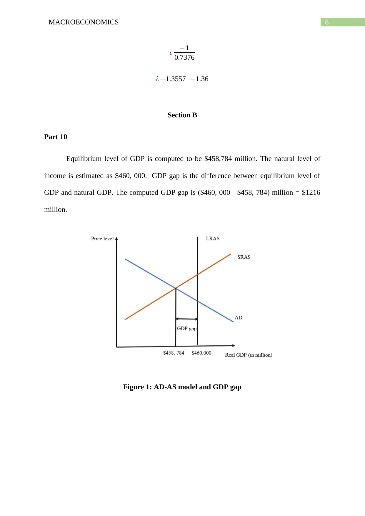
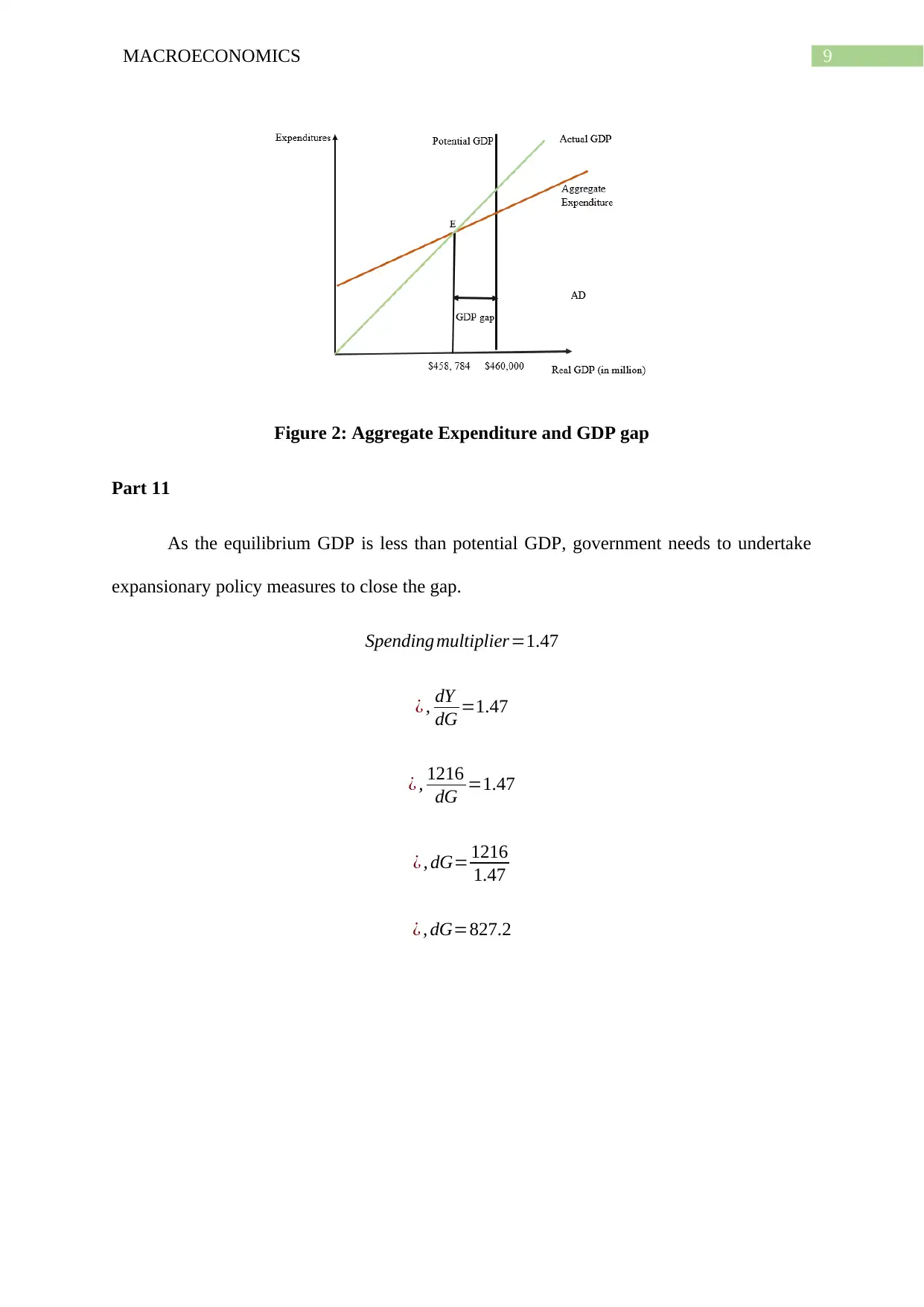
Macroeconomics Assignment: Economic Equilibrium and Policies
VerifiedAdded on 2022/12/22
|14
|1430
|1
Homework Assignment
AI Summary
This macroeconomics assignment solution analyzes an economy using given data on consumption, investment, government expenditure, exports, and imports. The solution calculates autonomous consumption, total savings, actual investment, unintended inventory investment, autonomous imports, autonomous net exports, and autonomous planned expenditure. It determines whether the economy is in equilibrium and calculates the equilibrium level of income. The assignment further explores the marginal leakage rate, expenditure multiplier, and tax multipliers. Section B delves into GDP gaps, expansionary fiscal and monetary policies, crowding-out effects, and the impact of currency depreciation on the economy, including the IS-LM model and exchange rate dynamics. The solution provides detailed calculations and explanations to understand macroeconomic concepts and policy implications.


1 out of 14
Related Documents


Your All-in-One AI-Powered Toolkit for Academic Success.
+13062052269
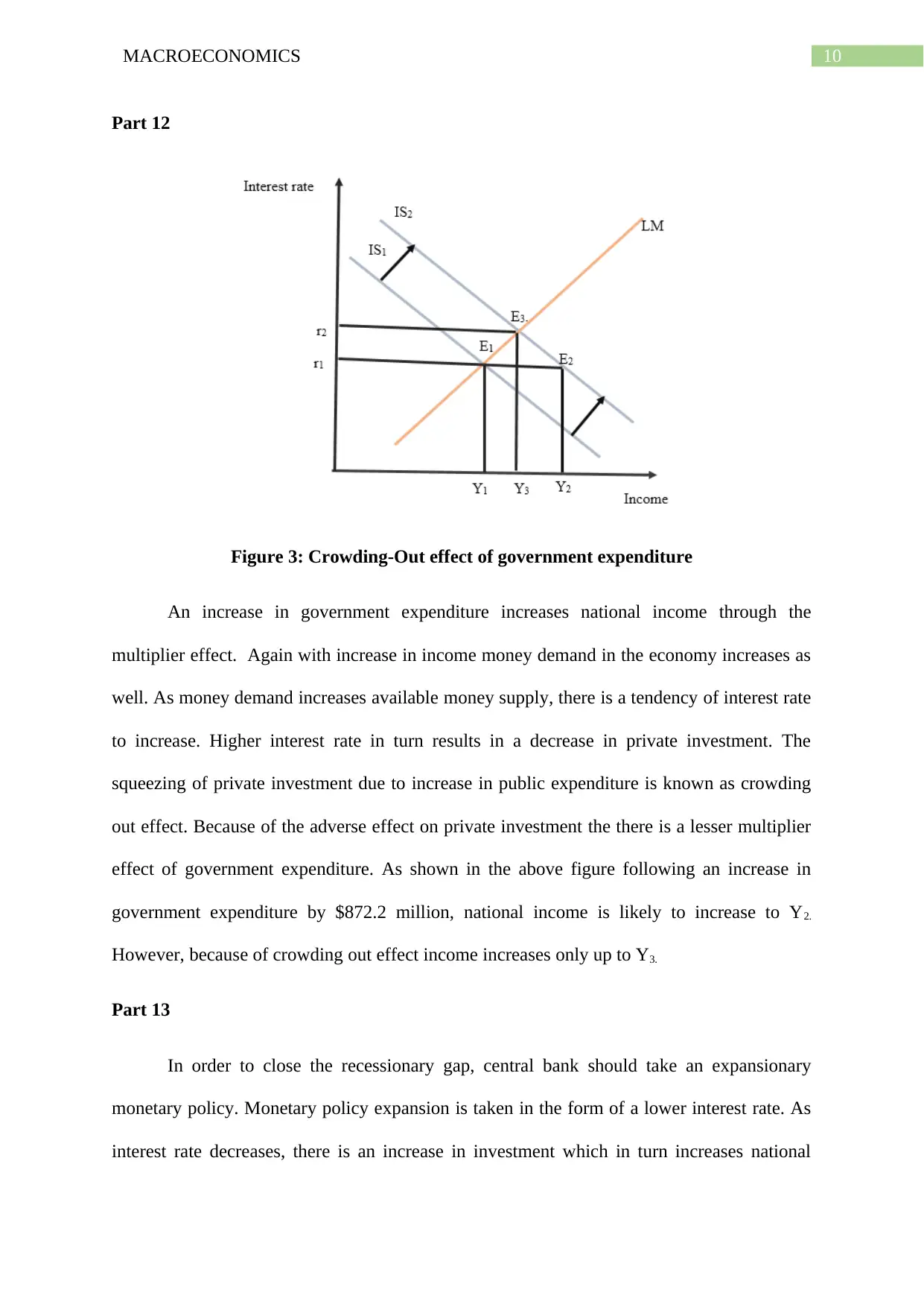
info@desklib.com
Available 24*7 on WhatsApp / Email
![[object Object]](/_next/static/media/star-bottom.7253800d.svg)
Copyright © 2020–2026 A2Z Services. All Rights Reserved. Developed and managed by ZUCOL.