MAE256 T1 2018: Regression Analysis of University Vice Chancellors

This assignment provides a detailed regression analysis of university vice chancellors' remuneration, exploring the relationships between remuneration, university rank, and student numbers. Several regression models are estimated, including linear and log-log specifications, to determine the impact of rank and student enrollment on remuneration. The analysis includes hypothesis testing using t-statistics and F-statistics to assess the statistical significance of the variables and the overall model fit. The assignment also investigates whether Vice Chancellors in Victoria are paid higher compared to other states using a dummy variable. The findings indicate the significance of rank and student numbers in explaining the variation in university vice chancellors' remuneration.

Running Head: MAE256 T1
MAE256 T1
Name of the Student
Name of the University
Course ID

1MAE256 T1
Table of Contents
Answer i...........................................................................................................................................2
Answer ii..........................................................................................................................................4
Answer iii.........................................................................................................................................5
Answer iv.........................................................................................................................................6
Answer v..........................................................................................................................................7
Answer vi.........................................................................................................................................8
Answer vii........................................................................................................................................9
Answer viii.....................................................................................................................................11
Answer ix.......................................................................................................................................11
Bibliography..................................................................................................................................13

2MAE256 T1
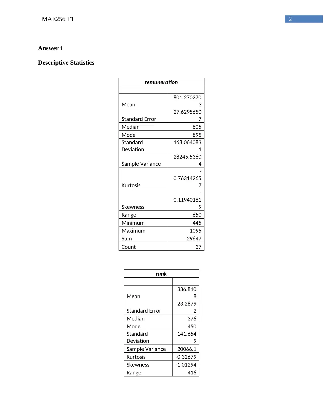
Answer i
Descriptive Statistics
remuneration
Mean
801.270270
3
Standard Error
27.6295650
7
Median 805
Mode 895
Standard
Deviation
168.064083
1
Sample Variance
28245.5360
4
Kurtosis
-
0.76314265
7
Skewness
-
0.11940181
9
Range 650
Minimum 445
Maximum 1095
Sum 29647
Count 37
rank
Mean
336.810
8
Standard Error
23.2879
2
Median 376
Mode 450
Standard
Deviation
141.654
9
Sample Variance 20066.1
Kurtosis -0.32679
Skewness -1.01294
Range 416

3MAE256 T1
Minimum 34
Maximum 450
Sum 12462
Count 37
studnum
Mean
38410.2702
7
Standard Error
6023.83362
1
Median 29214
Mode 26704
Standard
Deviation
36641.5494
4
Sample Variance 1342603145
Kurtosis
27.0045643
8
Skewness
4.85680684
6
Range 230347
Minimum 9899
Maximum 240246
Sum 1421180
Count 37
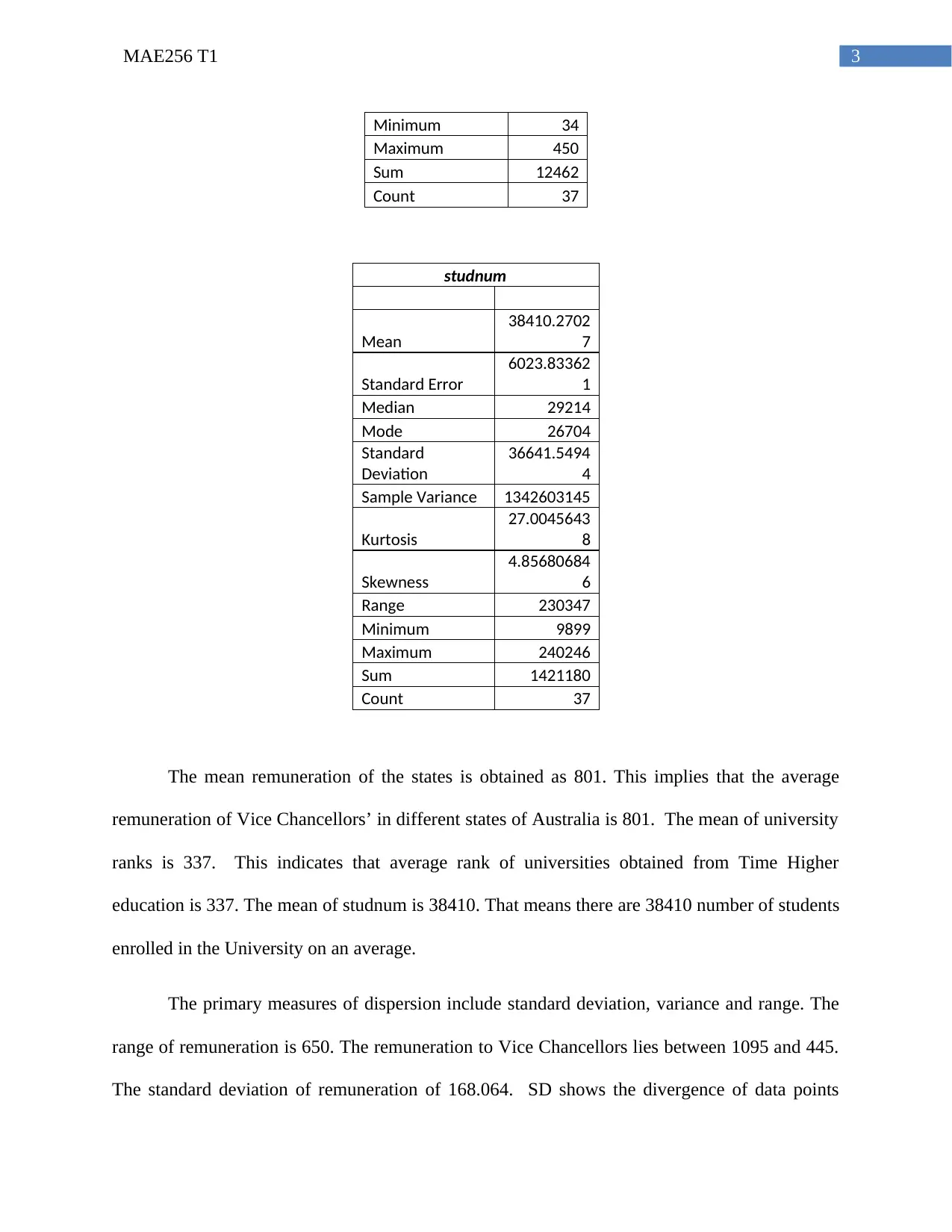
The mean remuneration of the states is obtained as 801. This implies that the average
remuneration of Vice Chancellors’ in different states of Australia is 801. The mean of university
ranks is 337. This indicates that average rank of universities obtained from Time Higher
education is 337. The mean of studnum is 38410. That means there are 38410 number of students
enrolled in the University on an average.
The primary measures of dispersion include standard deviation, variance and range. The
range of remuneration is 650. The remuneration to Vice Chancellors lies between 1095 and 445.
The standard deviation of remuneration of 168.064. SD shows the divergence of data points

4MAE256 T1
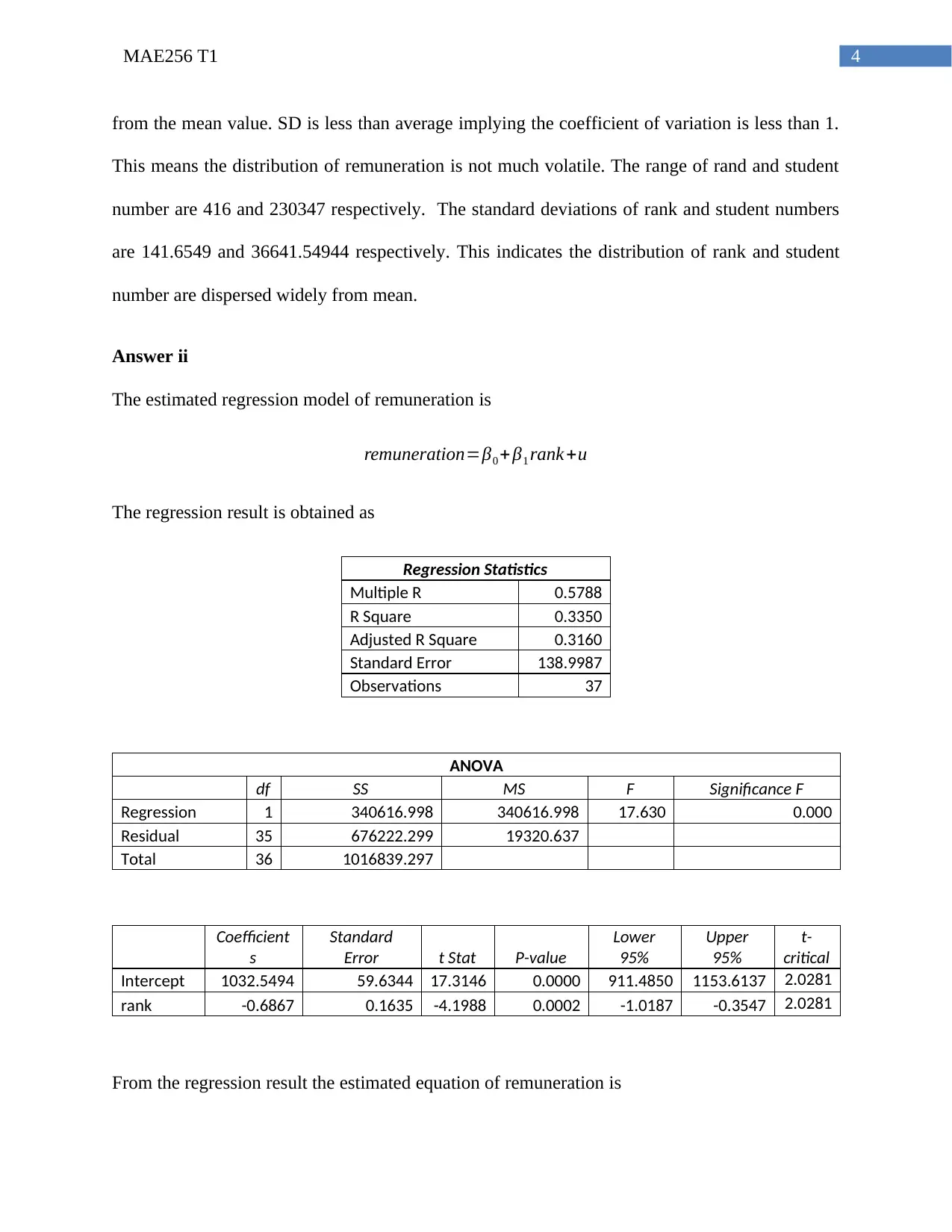
from the mean value. SD is less than average implying the coefficient of variation is less than 1.
This means the distribution of remuneration is not much volatile. The range of rand and student
number are 416 and 230347 respectively. The standard deviations of rank and student numbers
are 141.6549 and 36641.54944 respectively. This indicates the distribution of rank and student
number are dispersed widely from mean.
Answer ii
The estimated regression model of remuneration is
remuneration=β0 + β1 rank +u
The regression result is obtained as
Regression Statistics
Multiple R 0.5788
R Square 0.3350
Adjusted R Square 0.3160
Standard Error 138.9987
Observations 37
ANOVA
df SS MS F Significance F
Regression 1 340616.998 340616.998 17.630 0.000
Residual 35 676222.299 19320.637
Total 36 1016839.297
Coefficient
s
Standard
Error t Stat P-value
Lower
95%
Upper
95%
t-
critical
Intercept 1032.5494 59.6344 17.3146 0.0000 911.4850 1153.6137 2.0281
rank -0.6867 0.1635 -4.1988 0.0002 -1.0187 -0.3547 2.0281
From the regression result the estimated equation of remuneration is

5MAE256 T1
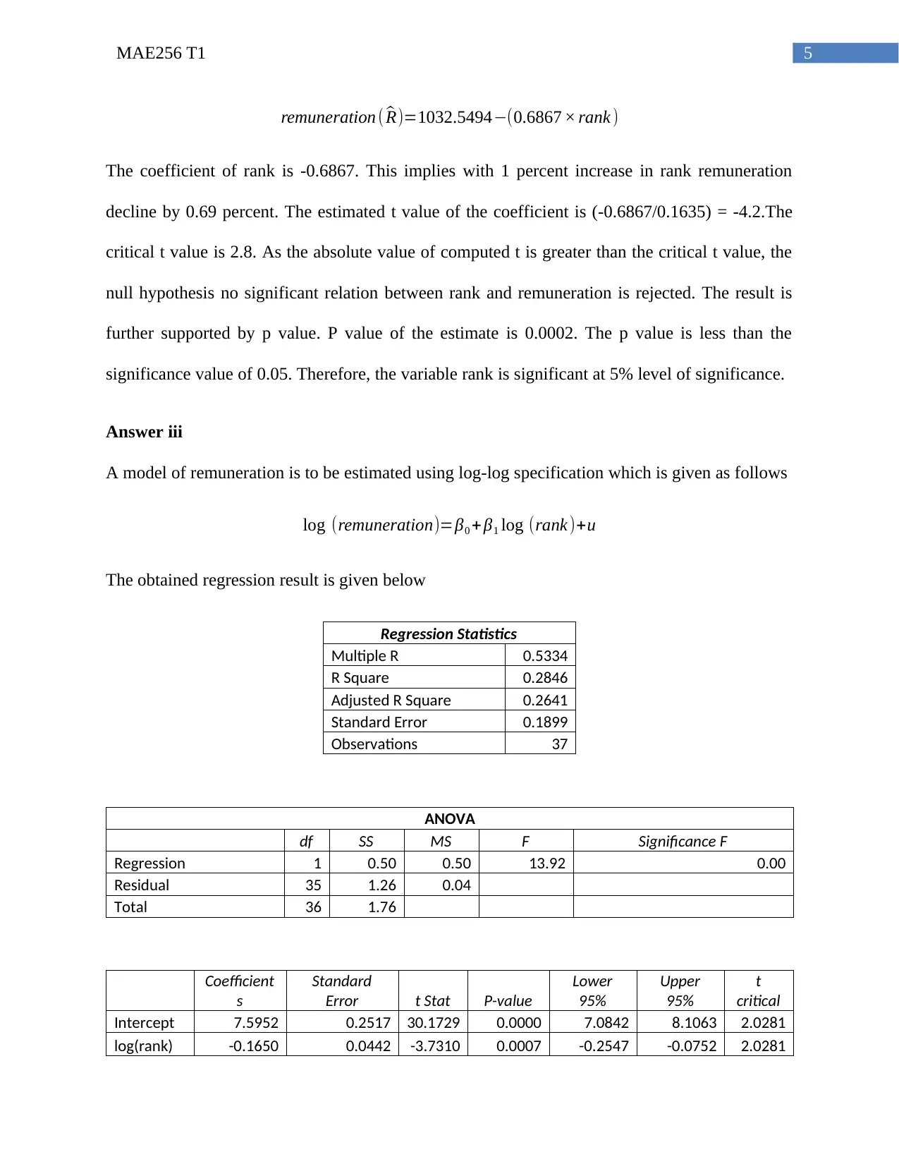
remuneration ( ^R)=1032.5494−(0.6867 × rank )
The coefficient of rank is -0.6867. This implies with 1 percent increase in rank remuneration
decline by 0.69 percent. The estimated t value of the coefficient is (-0.6867/0.1635) = -4.2.The
critical t value is 2.8. As the absolute value of computed t is greater than the critical t value, the
null hypothesis no significant relation between rank and remuneration is rejected. The result is
further supported by p value. P value of the estimate is 0.0002. The p value is less than the
significance value of 0.05. Therefore, the variable rank is significant at 5% level of significance.
Answer iii
A model of remuneration is to be estimated using log-log specification which is given as follows
log (remuneration)=β0 + β1 log (rank )+u
The obtained regression result is given below
Regression Statistics
Multiple R 0.5334
R Square 0.2846
Adjusted R Square 0.2641
Standard Error 0.1899
Observations 37
ANOVA
df SS MS F Significance F
Regression 1 0.50 0.50 13.92 0.00
Residual 35 1.26 0.04
Total 36 1.76
Coefficient
s
Standard
Error t Stat P-value
Lower
95%
Upper
95%
t
critical
Intercept 7.5952 0.2517 30.1729 0.0000 7.0842 8.1063 2.0281
log(rank) -0.1650 0.0442 -3.7310 0.0007 -0.2547 -0.0752 2.0281

6MAE256 T1
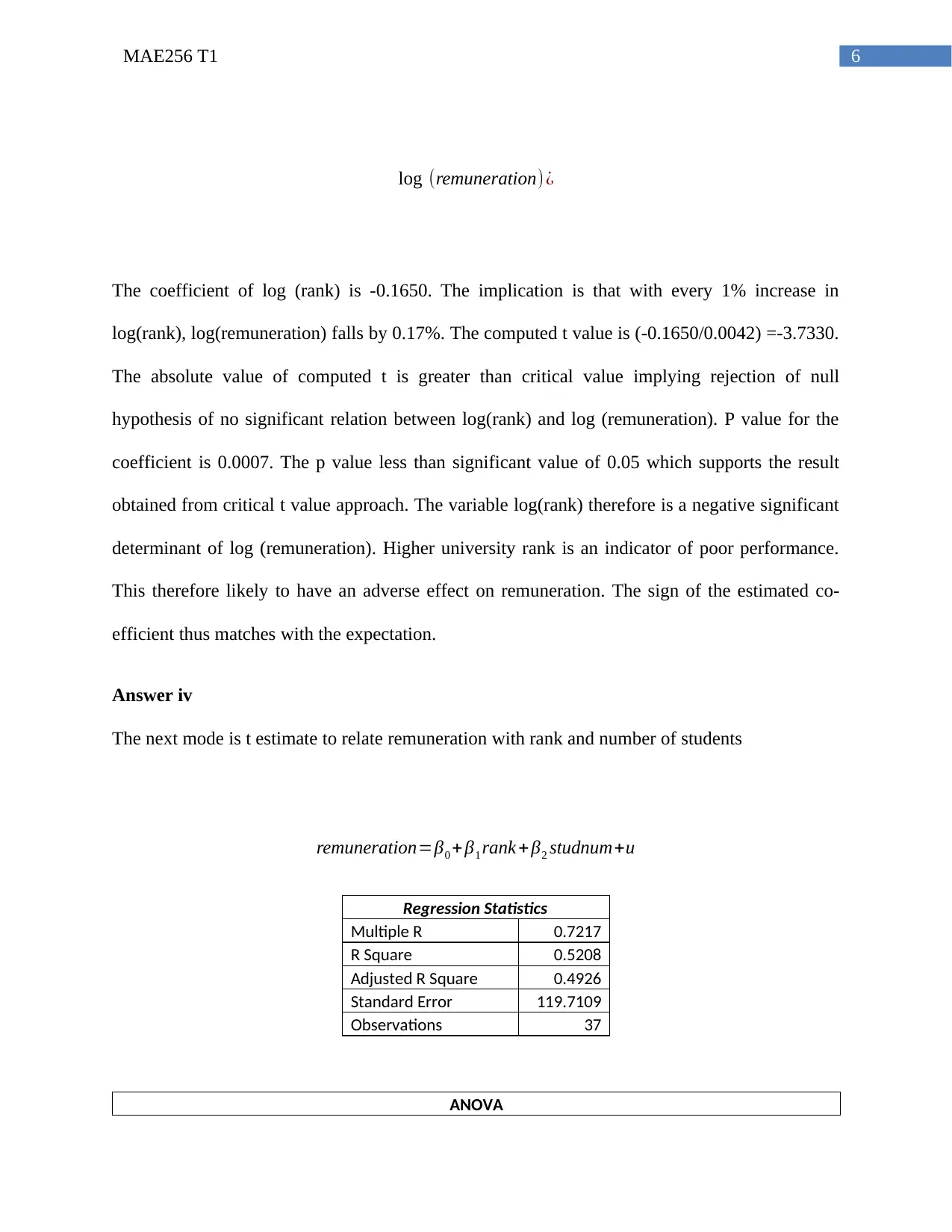
log (remuneration) ¿
The coefficient of log (rank) is -0.1650. The implication is that with every 1% increase in
log(rank), log(remuneration) falls by 0.17%. The computed t value is (-0.1650/0.0042) =-3.7330.
The absolute value of computed t is greater than critical value implying rejection of null
hypothesis of no significant relation between log(rank) and log (remuneration). P value for the
coefficient is 0.0007. The p value less than significant value of 0.05 which supports the result
obtained from critical t value approach. The variable log(rank) therefore is a negative significant
determinant of log (remuneration). Higher university rank is an indicator of poor performance.
This therefore likely to have an adverse effect on remuneration. The sign of the estimated co-
efficient thus matches with the expectation.
Answer iv
The next mode is t estimate to relate remuneration with rank and number of students
remuneration=β0 + β1 rank +β2 studnum+u
Regression Statistics
Multiple R 0.7217
R Square 0.5208
Adjusted R Square 0.4926
Standard Error 119.7109
Observations 37
ANOVA

7MAE256 T1
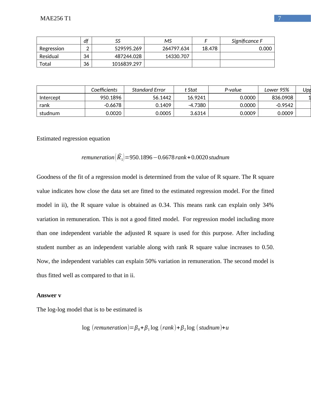
df SS MS F Significance F
Regression 2 529595.269 264797.634 18.478 0.000
Residual 34 487244.028 14330.707
Total 36 1016839.297
Coefficients Standard Error t Stat P-value Lower 95% Upp
Intercept 950.1896 56.1442 16.9241 0.0000 836.0908 1
rank -0.6678 0.1409 -4.7380 0.0000 -0.9542
studnum 0.0020 0.0005 3.6314 0.0009 0.0009
Estimated regression equation
remuneration ( ^R1 ) =950.1896−0.6678 rank + 0.0020 studnum
Goodness of the fit of a regression model is determined from the value of R square. The R square
value indicates how close the data set are fitted to the estimated regression model. For the fitted
model in ii), the R square value is obtained as 0.34. This means rank can explain only 34%
variation in remuneration. This is not a good fitted model. For regression model including more
than one independent variable the adjusted R square is used for this purpose. After including
student number as an independent variable along with rank R square value increases to 0.50.
Now, the independent variables can explain 50% variation in remuneration. The second model is
thus fitted well as compared to that in ii.
Answer v
The log-log model that is to be estimated is
log (remuneration)=β0 + β1 log (rank )+ β2 log ( studnum)+u

8MAE256 T1
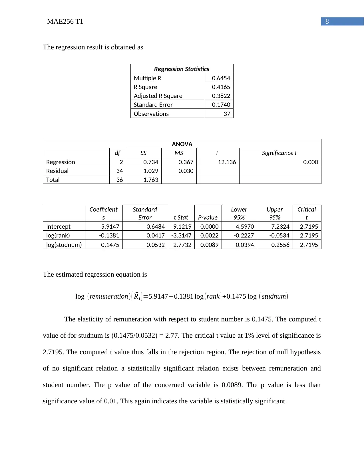
The regression result is obtained as
Regression Statistics
Multiple R 0.6454
R Square 0.4165
Adjusted R Square 0.3822
Standard Error 0.1740
Observations 37
ANOVA
df SS MS F Significance F
Regression 2 0.734 0.367 12.136 0.000
Residual 34 1.029 0.030
Total 36 1.763
Coefficient
s
Standard
Error t Stat P-value
Lower
95%
Upper
95%
Critical
t
Intercept 5.9147 0.6484 9.1219 0.0000 4.5970 7.2324 2.7195
log(rank) -0.1381 0.0417 -3.3147 0.0022 -0.2227 -0.0534 2.7195
log(studnum) 0.1475 0.0532 2.7732 0.0089 0.0394 0.2556 2.7195
The estimated regression equation is
log (remuneration) ( ^R1 ) =5.9147−0.1381 log ( rank ) +0.1475 log (studnum)
The elasticity of remuneration with respect to student number is 0.1475. The computed t
value of for studnum is (0.1475/0.0532) = 2.77. The critical t value at 1% level of significance is
2.7195. The computed t value thus falls in the rejection region. The rejection of null hypothesis
of no significant relation a statistically significant relation exists between remuneration and
student number. The p value of the concerned variable is 0.0089. The p value is less than
significance value of 0.01. This again indicates the variable is statistically significant.

9MAE256 T1
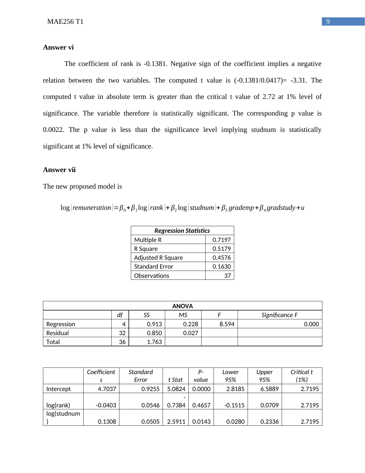
Answer vi
The coefficient of rank is -0.1381. Negative sign of the coefficient implies a negative
relation between the two variables. The computed t value is (-0.1381/0.0417)= -3.31. The
computed t value in absolute term is greater than the critical t value of 2.72 at 1% level of
significance. The variable therefore is statistically significant. The corresponding p value is
0.0022. The p value is less than the significance level implying studnum is statistically
significant at 1% level of significance.
Answer vii
The new proposed model is
log ( remuneration ) =β0 +β1 log ( rank ) + β2 log ( studnum ) + β3 grademp+β4 gradstudy +u
Regression Statistics
Multiple R 0.7197
R Square 0.5179
Adjusted R Square 0.4576
Standard Error 0.1630
Observations 37
ANOVA
df SS MS F Significance F
Regression 4 0.913 0.228 8.594 0.000
Residual 32 0.850 0.027
Total 36 1.763
Coefficient
s
Standard
Error t Stat
P-
value
Lower
95%
Upper
95%
Critical t
(1%)
Intercept 4.7037 0.9255 5.0824 0.0000 2.8185 6.5889 2.7195
log(rank) -0.0403 0.0546
-
0.7384 0.4657 -0.1515 0.0709 2.7195
log(studnum
) 0.1308 0.0505 2.5911 0.0143 0.0280 0.2336 2.7195

10MAE256 T1
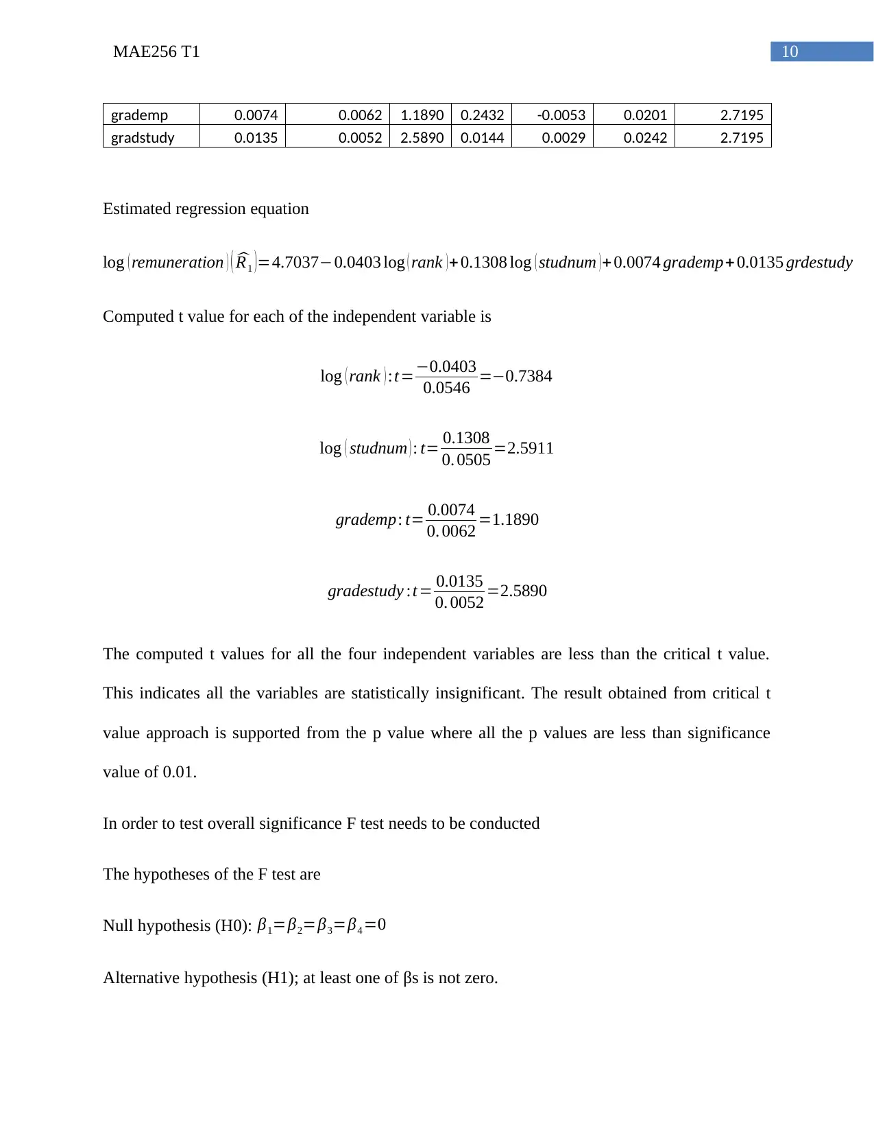
grademp 0.0074 0.0062 1.1890 0.2432 -0.0053 0.0201 2.7195
gradstudy 0.0135 0.0052 2.5890 0.0144 0.0029 0.0242 2.7195
Estimated regression equation
log ( remuneration ) ( ^R1 )=4.7037−0.0403 log ( rank ) + 0.1308 log ( studnum ) + 0.0074 grademp+ 0.0135 grdestudy
Computed t value for each of the independent variable is
log ( rank ) :t=−0.0403
0.0546 =−0.7384
log ( studnum ) : t= 0.1308
0. 0505 =2.5911
grademp: t= 0.0074
0. 0062 =1.1890
gradestudy :t= 0.0135
0. 0052 =2.5890
The computed t values for all the four independent variables are less than the critical t value.
This indicates all the variables are statistically insignificant. The result obtained from critical t
value approach is supported from the p value where all the p values are less than significance
value of 0.01.
In order to test overall significance F test needs to be conducted
The hypotheses of the F test are
Null hypothesis (H0): β1=β2=β3=β4 =0
Alternative hypothesis (H1); at least one of βs is not zero.

11MAE256 T1
F=
RSS
K
SSE
[n− ( k +1 )]
= Meanregrssion∑ of square
Mean squared error = MSR
MSE F4,32
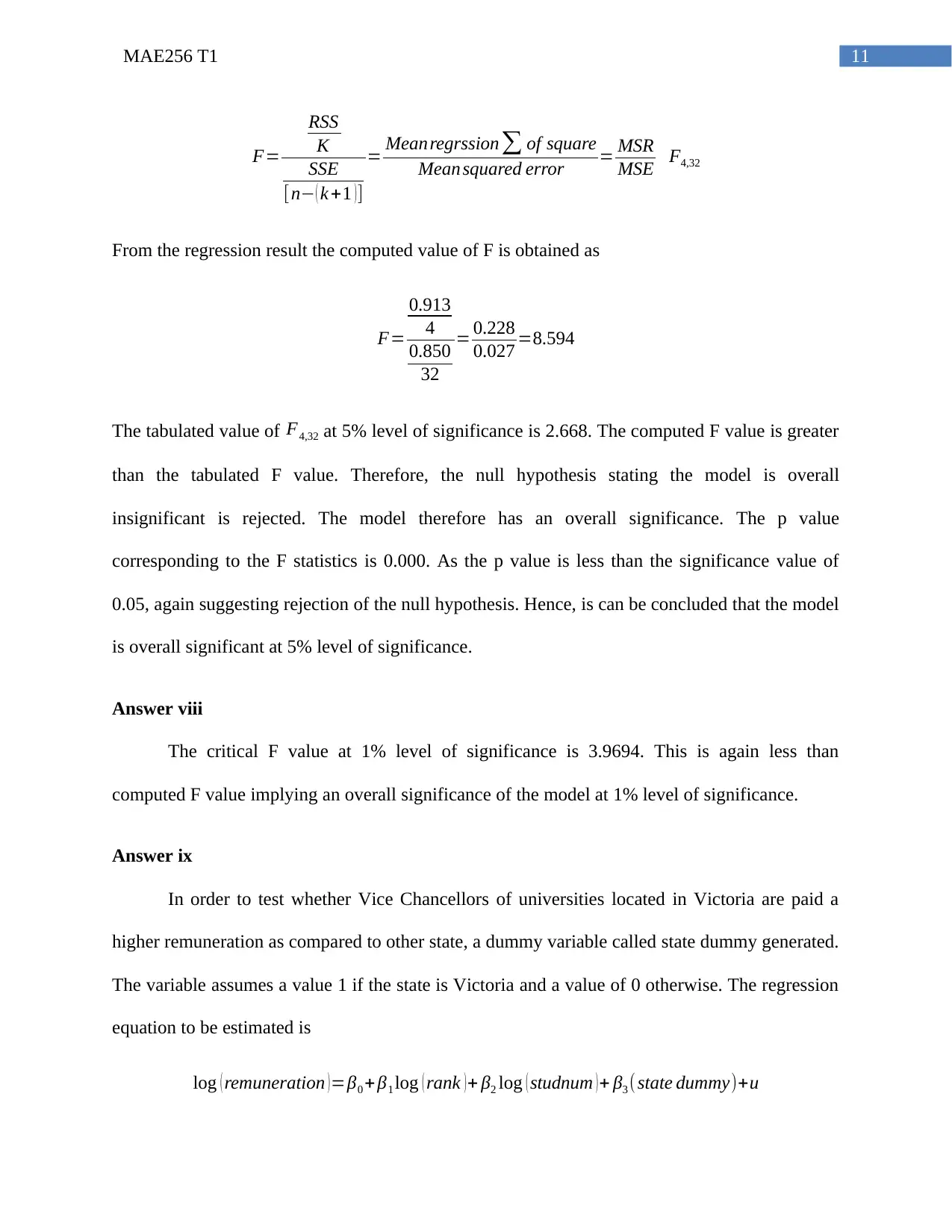
From the regression result the computed value of F is obtained as
F=
0.913
4
0.850
32
= 0.228
0.027 =8.594
The tabulated value of F4,32 at 5% level of significance is 2.668. The computed F value is greater
than the tabulated F value. Therefore, the null hypothesis stating the model is overall
insignificant is rejected. The model therefore has an overall significance. The p value
corresponding to the F statistics is 0.000. As the p value is less than the significance value of
0.05, again suggesting rejection of the null hypothesis. Hence, is can be concluded that the model
is overall significant at 5% level of significance.
Answer viii
The critical F value at 1% level of significance is 3.9694. This is again less than
computed F value implying an overall significance of the model at 1% level of significance.
Answer ix
In order to test whether Vice Chancellors of universities located in Victoria are paid a
higher remuneration as compared to other state, a dummy variable called state dummy generated.
The variable assumes a value 1 if the state is Victoria and a value of 0 otherwise. The regression
equation to be estimated is
log ( remuneration )=β0 + β1 log ( rank )+ β2 log ( studnum )+ β3 ( state dummy)+u