Management Science: Regression and Hypothesis Testing Solutions

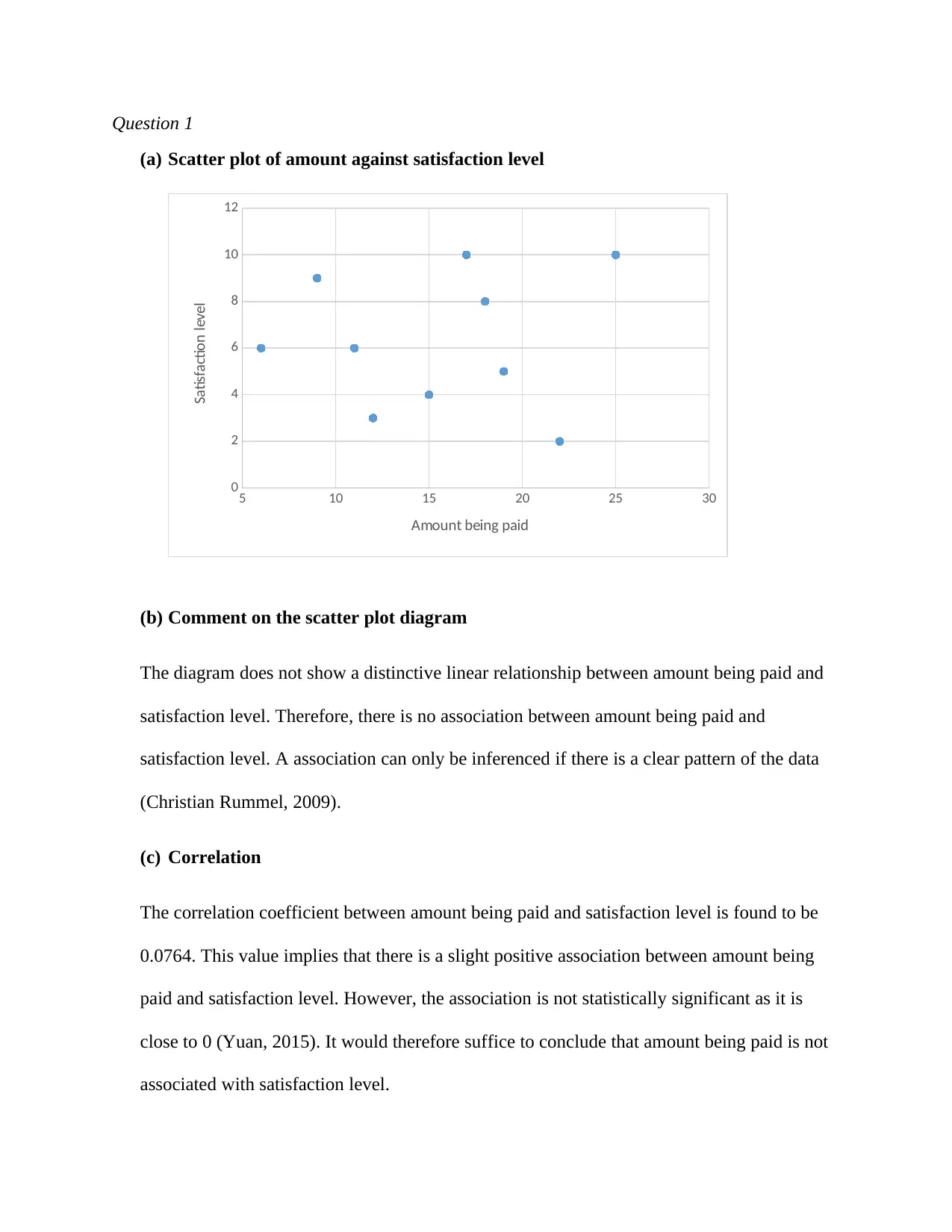
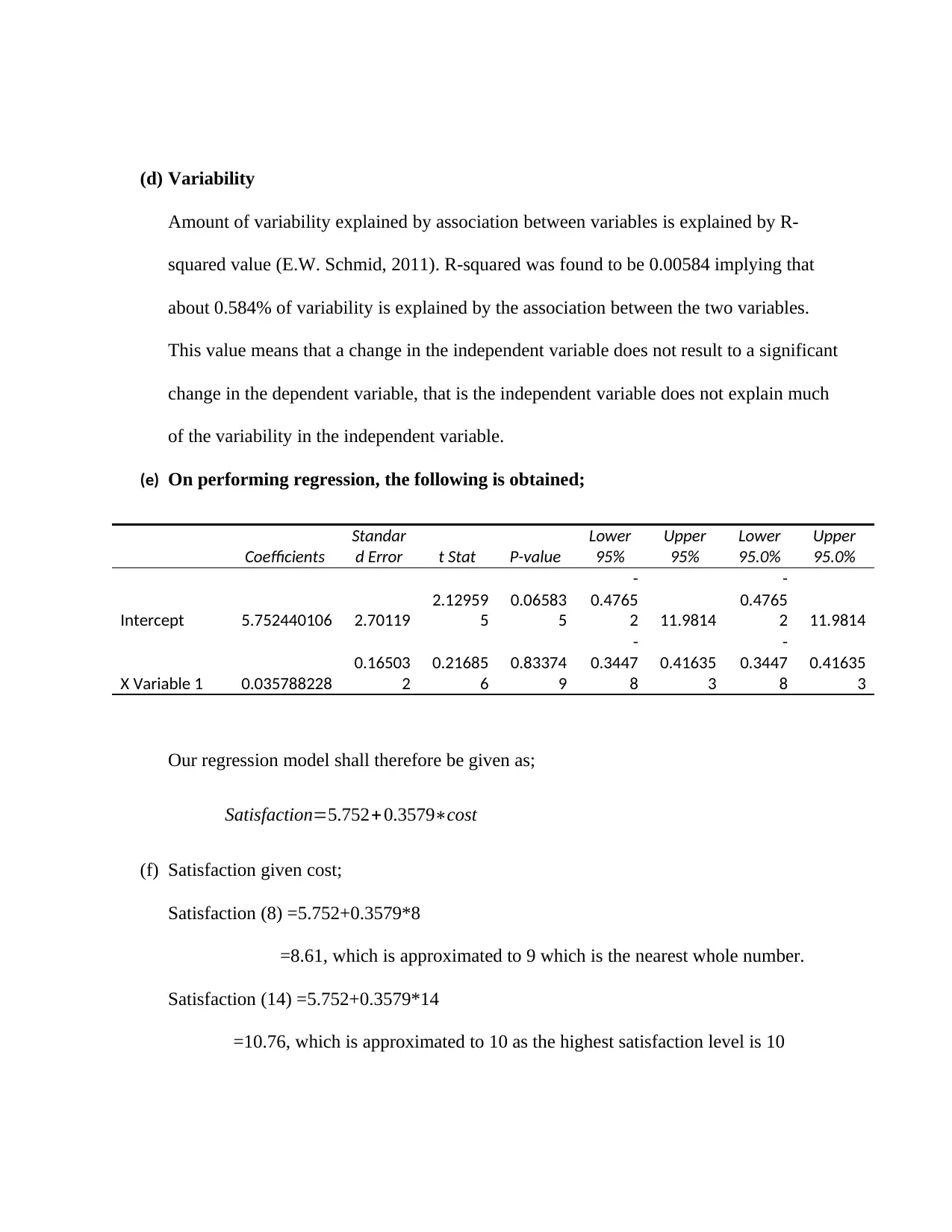
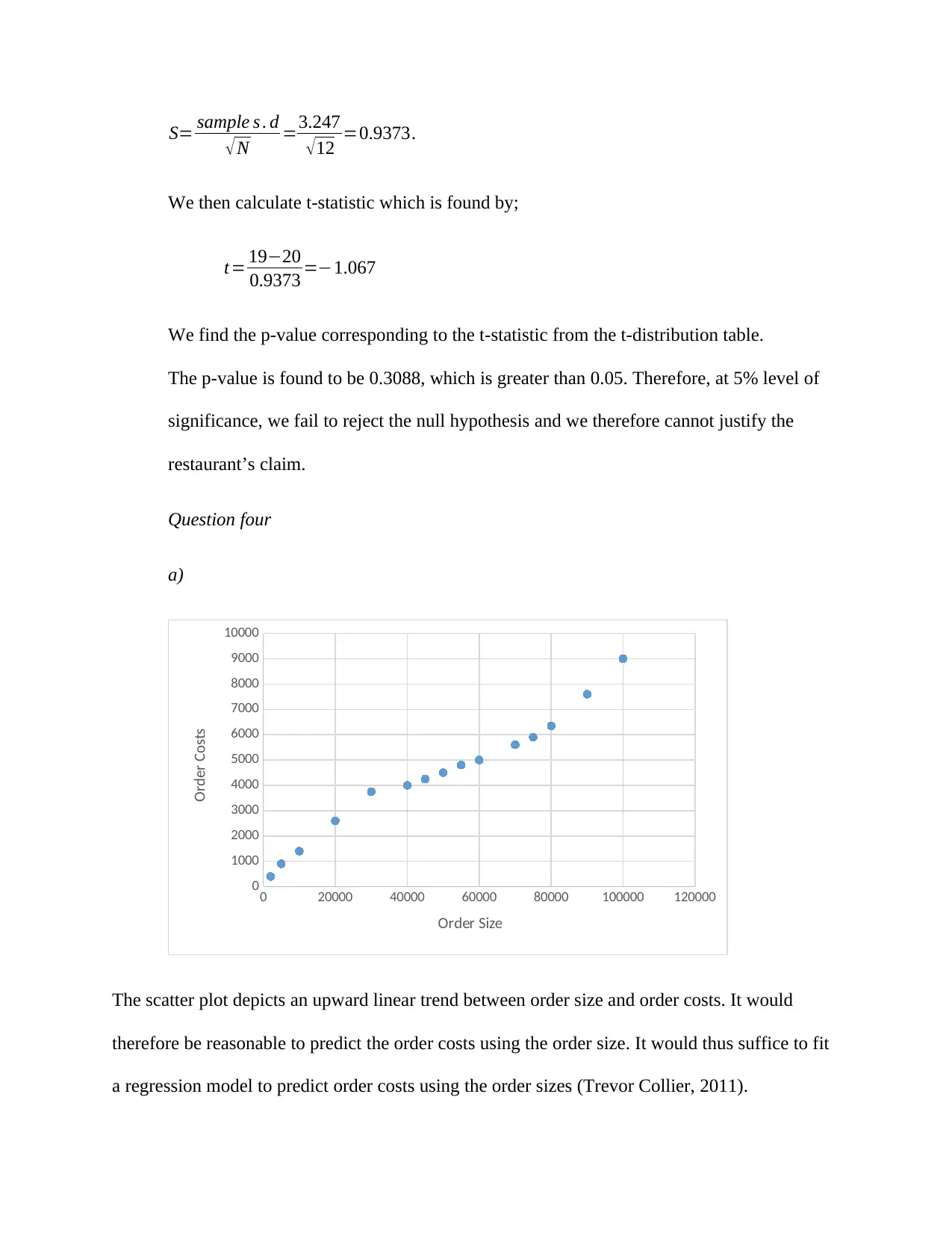
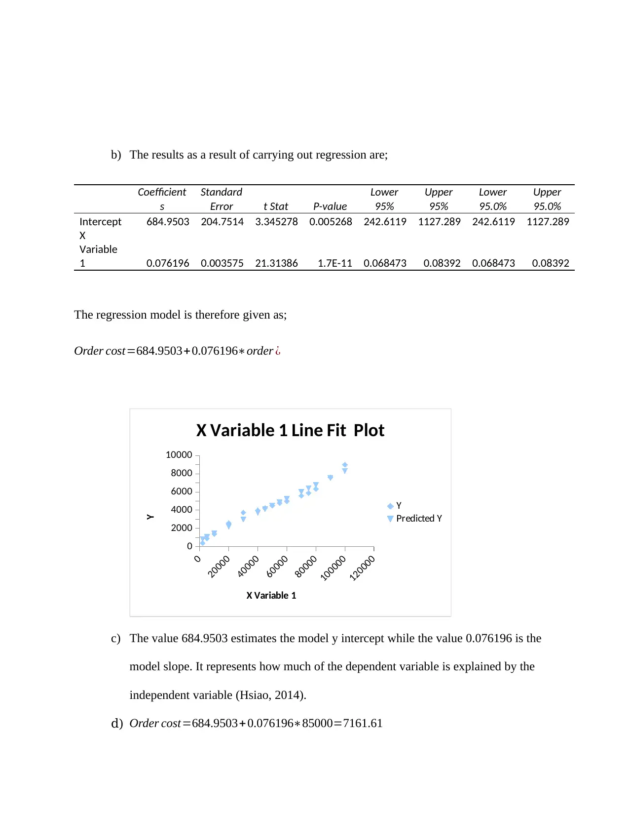
This assignment solution covers several statistical analyses within the context of Management Science. It includes the creation and interpretation of a scatter plot to assess the relationship between amount paid and satisfaction level, calculation and explanation of the correlation coefficient and R-squared value, and the derivation and application of a regression model to predict satisfaction levels based on cost. The solution also addresses hypothesis testing, including a test of proportions related to credit union mergers and a t-test to evaluate restaurant claims, along with chi-square tests to analyze the impact of health promotion campaigns and the relationship between living arrangements and exercise habits. Finally, it covers point estimates, confidence intervals, and hypothesis testing for comparing customer satisfaction ratings between two companies. Each question provides detailed calculations, interpretations, and conclusions based on statistical significance.

Question 1
(a) Scatter plot of amount against satisfaction level
5 10 15 20 25 30
0
2
4
6
8
10
12
Amount being paid
Satisfaction level
(b) Comment on the scatter plot diagram
The diagram does not show a distinctive linear relationship between amount being paid and
satisfaction level. Therefore, there is no association between amount being paid and
satisfaction level. A association can only be inferenced if there is a clear pattern of the data
(Christian Rummel, 2009).
(c) Correlation
The correlation coefficient between amount being paid and satisfaction level is found to be
0.0764. This value implies that there is a slight positive association between amount being
paid and satisfaction level. However, the association is not statistically significant as it is
close to 0 (Yuan, 2015). It would therefore suffice to conclude that amount being paid is not
associated with satisfaction level.

(d) Variability
Amount of variability explained by association between variables is explained by R-
squared value (E.W. Schmid, 2011). R-squared was found to be 0.00584 implying that
about 0.584% of variability is explained by the association between the two variables.
This value means that a change in the independent variable does not result to a significant
change in the dependent variable, that is the independent variable does not explain much
of the variability in the independent variable.
(e) On performing regression, the following is obtained;
Coefficients
Standar
d Error t Stat P-value
Lower
95%
Upper
95%
Lower
95.0%
Upper
95.0%
Intercept 5.752440106 2.70119
2.12959
5
0.06583
5
-
0.4765
2 11.9814
-
0.4765
2 11.9814
X Variable 1 0.035788228
0.16503
2
0.21685
6
0.83374
9
-
0.3447
8
0.41635
3
-
0.3447
8
0.41635
3
Our regression model shall therefore be given as;
Satisfaction=5.752+ 0.3579∗cost
(f) Satisfaction given cost;
Satisfaction (8) =5.752+0.3579*8
=8.61, which is approximated to 9 which is the nearest whole number.
Satisfaction (14) =5.752+0.3579*14
=10.76, which is approximated to 10 as the highest satisfaction level is 10

Satisfaction (23) =5.752+0.3579*23
=13.98, which is approximated to 10 as the highest satisfaction level is 10
Question two
The task is to test whether at 1% level of significance, the members of credit union B are equally
divided on the merger. We test whether the assumed proportion is equal to the proportion
resultant from the survey.
Our hypothesis is;
H0: The calculated proportion is different from 0.5.
H1: The calculated proportion equals 0.5.
We first calculate the standard deviation which is given as;
ẟ=√ ( p∗1− p
n ), where p=0.5
ẟ=√ [ 0.5∗0.5
400 ]
ẟ= √ 0.000625=0.025 ,
We then calculate the sample proportion P, which is 219
400 =0.5475.
We then calculate the test statistic defined as;
Z=(P− p) /ẟ
Z=(0.5−0.5475)/0.025

Z=−1.9
We find the p-value by checking the corresponding value of the Z-score from the normal
distribution table;
We find a p-value of 0.02872. Since the p-value is greater than the significance value 0.01
(Fraser, 2017), we reject the null hypothesis that the observed proportion is different from 0.05.
We therefore conclude that there is enough evidence at the 1% level of significance to support
the claim of the general manager of Credit Union B.
Question three
a) The mean of the sample is found to be 19%.
We test whether the mean is less than 20%. We therefore test the following hypothesis;
H0: The mean is not less than 20%.
H1: The mean is less than 20%.
The test statistic is calculated as;
t= 19−20
3
√ 12
=−1.155
We find the p-value corresponding to the t-statistic from the t-distribution table.
The p-value is found to be 0.2726, which is greater than 0.05. Therefore, at 5% level of
significance, we fail to reject the null hypothesis and we therefore cannot justify the
restaurant’s claim.
b) Assuming, the population standard deviation is not known, we first find the sample
standard deviation (3.247) then find the estimated standard error of the mean, S, which is
calculated as;

S= sample s . d
√N =3.247
√12 =0.9373.
We then calculate t-statistic which is found by;
t= 19−20
0.9373 =−1.067
We find the p-value corresponding to the t-statistic from the t-distribution table.
The p-value is found to be 0.3088, which is greater than 0.05. Therefore, at 5% level of
significance, we fail to reject the null hypothesis and we therefore cannot justify the
restaurant’s claim.
Question four
a)
0 20000 40000 60000 80000 100000 120000
0
1000
2000
3000
4000
5000
6000
7000
8000
9000
10000
Order Size
Order Costs
The scatter plot depicts an upward linear trend between order size and order costs. It would
therefore be reasonable to predict the order costs using the order size. It would thus suffice to fit
a regression model to predict order costs using the order sizes (Trevor Collier, 2011).

b) The results as a result of carrying out regression are;
Coefficient
s
Standard
Error t Stat P-value
Lower
95%
Upper
95%
Lower
95.0%
Upper
95.0%
Intercept 684.9503 204.7514 3.345278 0.005268 242.6119 1127.289 242.6119 1127.289
X
Variable
1 0.076196 0.003575 21.31386 1.7E-11 0.068473 0.08392 0.068473 0.08392
The regression model is therefore given as;
Order cost=684.9503+0.076196∗order ¿
0
20000
40000
60000
80000
100000
120000
0
2000
4000
6000
8000
10000
X Variable 1 Line Fit Plot
Y
Predicted Y
X Variable 1
Y
c) The value 684.9503 estimates the model y intercept while the value 0.076196 is the
model slope. It represents how much of the dependent variable is explained by the
independent variable (Hsiao, 2014).
d) Order cost=684.9503+ 0.076196∗85000=7161.61

e) The model shows an upward linear trend. It is therefore easy to predict values of the y
variable given any value of the x variable. Therefore, it would be valid to use the
model to produce a price estimate requiring the production of 120,000 units.
Question five
a) We test the hypothesis;
H0: p1=0.60, p2=0.25, p3=0.15,
H1: H0 is not true
The test statistics is;
We first carry out a test to assess whether the sample size is large enough to carry out a
chi-square test. Specifically, we need to check min (np0, np1, ..., npk) > 5. The sample size
here is n=470 and the proportions specified in the null hypothesis are 0.60, 0.25 and 0.15.
Thus, min (470(0.60), 470(0.25), 470(0.15)) = min (282, 117.5, 70.5) = 70.5. Since the
minimum off npk is greater than 5, it suffices that a chi square test will be appropriate for
this task.
The test statistic is computed as;
( 256−282 )2
282 + ( 125−117.5 )2
117.5 + ( 90−70.5 )2
70.5
¿ 2.59+0.48+5.39=8.46
We compare the value 8.46 to the 5% critical value (5.99). Since our test statistic is
greater than the critical value we reject the null hypothesis (Michael R. Kosorok, 2010).

Therefore, the distribution of responses to the exercise question following the
implementation of the health promotion campaign was not the same as the distribution
prior.
b) We testing the following hypothesis;
H0: There is no relationship between living arrangement and exercise.
H1: There is a relationship between living arrangements and exercise.
We calculate the test statistic using the formula;
We compute the expected frequencies using the formula;
Expected Frequency = (Row Total * Column Total)/N.
No Regular
Exercise
Sporadic
Exercise
Regular
Exercise
Total
Dormitory 32
(48.8)
30
(23.9)
28
(17.2)
90
On-Campus
Apartment
74
(97.7)
64
(47.9)
42
(34.5)
180
Off-Campus
Apartment
110
(81.4)
25
(39.9)
15
(28.7)
150
At Home 39
(27.1)
6
(13.3)
5
(9.6)
50
Total 255 125 90 470
The test statistic is computed as;
( 32−48.8 ) 2
48.8 + ( 30−23.9 ) 2
23.9 + ( 28−17.2 ) 2
17.2 + ( 7448.8 ) 2
48.8 + ( 64−47.9 ) 2
47.9 + ( 42−34.5 ) 2
34.5 + ( 110−81.4 ) 2
81.4 + ( 25−39.9 ) 2
39.9 + ( 15−28
28.7

¿ 5.78+1.58+6.78+5.75+5.41+1.63+10.05+ 5.58+ 6.54+5.23+4.01+2.20
¿ 60.5
We compare the test statistic to the 5% critical value at 6 degrees of freedom (12.59). Since 60.5
is greater than 12.59, we reject the null hypothesis that there is no relationship between living
arrangements and exercise and conclude that there is a relationship between living arrangements
and exercise.
Question six
a) Point estimate and 99% confidence interval for difference in mean.
The point estimate for the difference in the means of the two populations is;
3.51−3.24=0.27
The confidence interval for the difference of two population means when standard deviation
is known is given by;
The standard error is given as;
√ ( 0.51 )2
174 + ( 0.52 )2
355 =0.0475.
Therefore, the 99% confidence interval is;
0.27 ± 2.58 ( 0.0474 )
¿( 0.15,0.39)

b) We test the hypothesis;
H0: Company ABC does not have a higher customer satisfaction rating than company
XYZ.
H1: Company ABC has a higher customer satisfaction rating than company XYZ.
We calculate the test statistic as;
Z= 0.27
√ 0.512
174 + 0.522
355
= 0.27
0.0474 =5.696
Since 5.696 is greater than 2.58 (Kinney, 2009), we reject the null hypothesis and
conclude that company ABC has a higher customer satisfaction rating than company
XYZ.

References
Christian Rummel, Gerold Baier, Markus Müller, 2009. The influence of static correlations on multivariate
correlation analysis. 166(2), pp.20.-Question 1b
Schmid, K.H. Hoffmann., 2011. Test of a least-squares variational method for non-relativistic scattering.
175, pp.6.-Question 1d
Fraser, D., 2017. p -Values: The Insight to Modern Statistical Inference. Annual Review of Statistics and
Its Application, 4, pp.5.-Question 2
Hsiao, C., 2014. Simple Regression with Variable Intercepts.pp.3.-Question 4c
Kinney, J. J., 2009. A Probability and Statistics Companion || Continuous Probability Distributions: Sums,
the Normal Distribution, and the Central Limit Theorem; Bivariate Random Variables. pp.22.-
Question 6b
Michael R. Kosorok, R. Q., 2010. Exact simultaneous confidence bands for a collection of univariate
polynomials in regression analysis. 18, pp.7.-Question 5a
Trevor Collier, Andrew L. Johnson, John Ruggiero, 2011. Technical efficiency estimation with multiple
inputs and multiple outputs using regression analysis. 208, pp.8.-Question 4a
Yuan, Naiming, Fu, Zuntao, Zhang, Huan, 2015. A New Method for Analyzing Correlations in Complex
System. 5, pp.6.-Question 1c

Appendix
Regression analysis output question 1 e
SUMMARY OUTPUT
Regression Statistics
Multiple R 0.076822
R Square 0.005902
Adjusted R
Square -0.11836
Standard
Error 3.034442
Observation
s 10
ANOVA
df SS MS F
Significan
ce F
Regression 1 0.437312
0.43731
2
0.04749
3 0.83294
Residual 8 73.66269
9.20783
6
Total 9 74.1
Coefficien
ts
Standard
Error t Stat P-value
Lower
95%
Upper
95%
Lower
95.0%
Upper
95.0%
Intercept 5.729271 2.789128
2.05414
5 0.07403 -0.70247
12.1610
1
-
0.7024
7
12.1610
1
X Variable 1 0.03706 0.170056 0.21793 0.83294 -0.35509 0.42921
-
0.3550
9 0.42921
RESIDUAL OUTPUT
Observatio
n
Predicted
Y
Residual
s
1 6.136935 -0.13693
2 6.396357 1.603643
3 6.359296 3.640704