Managerial Economics: Demand, Cost, and Market Structures Analysis

This managerial economics assignment explores various microeconomic concepts. Part 1 focuses on demand analysis, including the estimation of a demand function, statistical significance of coefficients, and elasticity calculations. Part 2 delves into the relationship between total, average, and marginal product, discussing the stages of production. Part 3 examines cost analysis, including explicit and implicit costs, and revenue and profit maximization. Finally, Part 4 analyzes monopoly market structures, including reasons for their existence and examples of price discrimination in Malaysia, such as in the electricity sector. The assignment provides detailed calculations, explanations, and examples to illustrate these economic principles.

Running Head: MANAGERIAL ECONOMICS
Managerial Economics
Name of the Student
Name of the University
Course ID

1MANAGERIAL ECONOMICS
Table of Contents
Part 1................................................................................................................................................2
Answer a......................................................................................................................................2
Answer b......................................................................................................................................5
Part 2................................................................................................................................................7
Part 3................................................................................................................................................9
Answer a......................................................................................................................................9
Answer b....................................................................................................................................10
Answer c....................................................................................................................................12
Part 4..............................................................................................................................................15
Reasons for existence of monopolies........................................................................................15
Answer b....................................................................................................................................16
Answer c....................................................................................................................................17
Reference list.................................................................................................................................18

2MANAGERIAL ECONOMICS
Part 1
Answer a
The demand function for Multipurpose Double-Sided Magic pan is given as
QM =250+30 Y +10 A +5 PT −10 PM
QM: Quantity of Magic Pan demanded
PM: Price per unit of Magic Pan
PT: Price per unit of another brand of pan
Y: Income level per household
A: Advertising expenditure
i)
In the demand equation, coefficient of income has a positive sign. The microeconomic
theory of demand suggests that for a normal good, an increase in income leads to an increases in
demand. The income coefficient thus has the expected sign. Firms promote their product through
advertising. The adverting thus likely to have a positive impact on demand. The coefficient of
advertising here found to have a positive sign. For substitute goods, demand of a product
changes in response to change in price of the substitute good. Price of one good has a positive
effect on demand of the substitute. Coefficient of price of another band of pan has a positive
sign. Sign of the estimated coefficient thus goes in line with economic theory. Lastly, own price
of the magic pan has a negative sign. This is again supported by economic theory of law of
demand which depicts an inverse relation between demand and own price.

3MANAGERIAL ECONOMICS
ii)
The value of R square is given as 0.87. The R square value is high and close to 1. This
means that own price, price of another brand of pan, income level and advertising together
explain 87% variation in the demand of quantity demanded of Magic Pan. The R square is a
measure of goodness of fit. Based on the high value of R square, the estimated equation can be
expected.
iii)
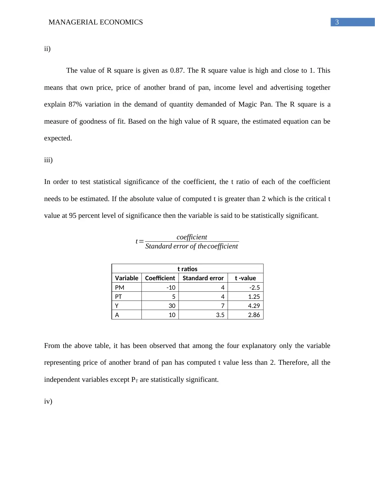
In order to test statistical significance of the coefficient, the t ratio of each of the coefficient
needs to be estimated. If the absolute value of computed t is greater than 2 which is the critical t
value at 95 percent level of significance then the variable is said to be statistically significant.
t= coefficient
Standard error of thecoefficient
t ratios
Variable Coefficient Standard error t -value
PM -10 4 -2.5
PT 5 4 1.25
Y 30 7 4.29
A 10 3.5 2.86
From the above table, it has been observed that among the four explanatory only the variable
representing price of another brand of pan has computed t value less than 2. Therefore, all the
independent variables except PT are statistically significant.
iv)

4MANAGERIAL ECONOMICS
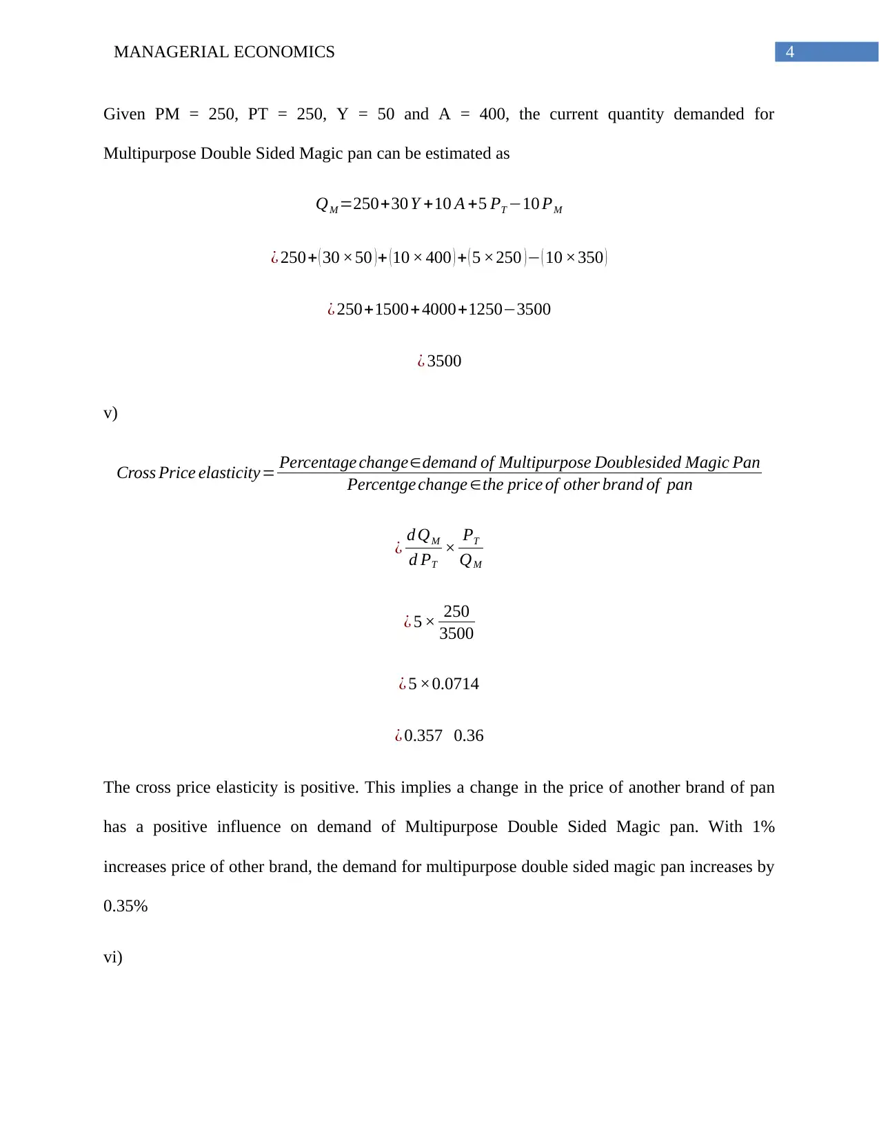
Given PM = 250, PT = 250, Y = 50 and A = 400, the current quantity demanded for
Multipurpose Double Sided Magic pan can be estimated as
QM =250+30 Y +10 A +5 PT −10 PM
¿ 250+ ( 30 ×50 ) + ( 10 × 400 ) + ( 5 ×250 ) − ( 10 ×350 )
¿ 250+1500+4000+1250−3500
¿ 3500
v)
Cross Price elasticity= Percentage change∈demand of Multipurpose Doublesided Magic Pan
Percentge change ∈the price of other brand of pan
¿ d QM
d PT
× PT
QM
¿ 5 × 250
3500
¿ 5 ×0.0714
¿ 0.357 0.36
The cross price elasticity is positive. This implies a change in the price of another brand of pan
has a positive influence on demand of Multipurpose Double Sided Magic pan. With 1%
increases price of other brand, the demand for multipurpose double sided magic pan increases by
0.35%
vi)

5MANAGERIAL ECONOMICS
Income elasticity= Percentage change∈demand of Multipurpose Doublesided Magic Pan
Percentge change∈income level per houehold
¿ d QM
dY × Y
QM
¿ 30 × 40
3500
¿ 30 ×0.0143
¿ 0.429 0.43
The income elasticity is less than 1. That is in response to a change in income, change in
demand is proportionately less than the corresponding change in income. This is the case of
necessity good.
vii)
Confidence interval for quantity demanded
^QM ± t0.05 × Standard error
¿ 3500 ± ( 2 × 9.50 )
¿ 3500 ±19
¿( 3481, 3519)
Answer b
i)
The model of kinked demand curve in an oligopoly market developed by Paul M. Sweezy
is based on the following assumption

6MANAGERIAL ECONOMICS
 The model assumes presence of a few firms in the oligopolistic market
 The few firms in the market are selling a product that is close substitute to each other.
 The product quality remains same and the firms do not engage in advertising
 There is set of price for the product that has been already decided and prevails in the
market.
 Each firm has a belief that if it lowers its price then rivals will immediately follow the
same. However, the same does not happen when it increases price (Fine, 2016). If one
firm increases price the others keep their prices same to make their product relatively
cheaper. The asymmetry in the reaction pattern of firms make the demand curve kinked
at the existing market price.
ii)
Because of the kinked demand curve, firms in the oligopoly market face a price rigidity. On the
inked demand curve, slope of the demand curve differs under condition of price increase or price
decrease. At price above the prevailing price the demand curve is highly elastic while below this
price the demand is inelastic.

7MANAGERIAL ECONOMICS
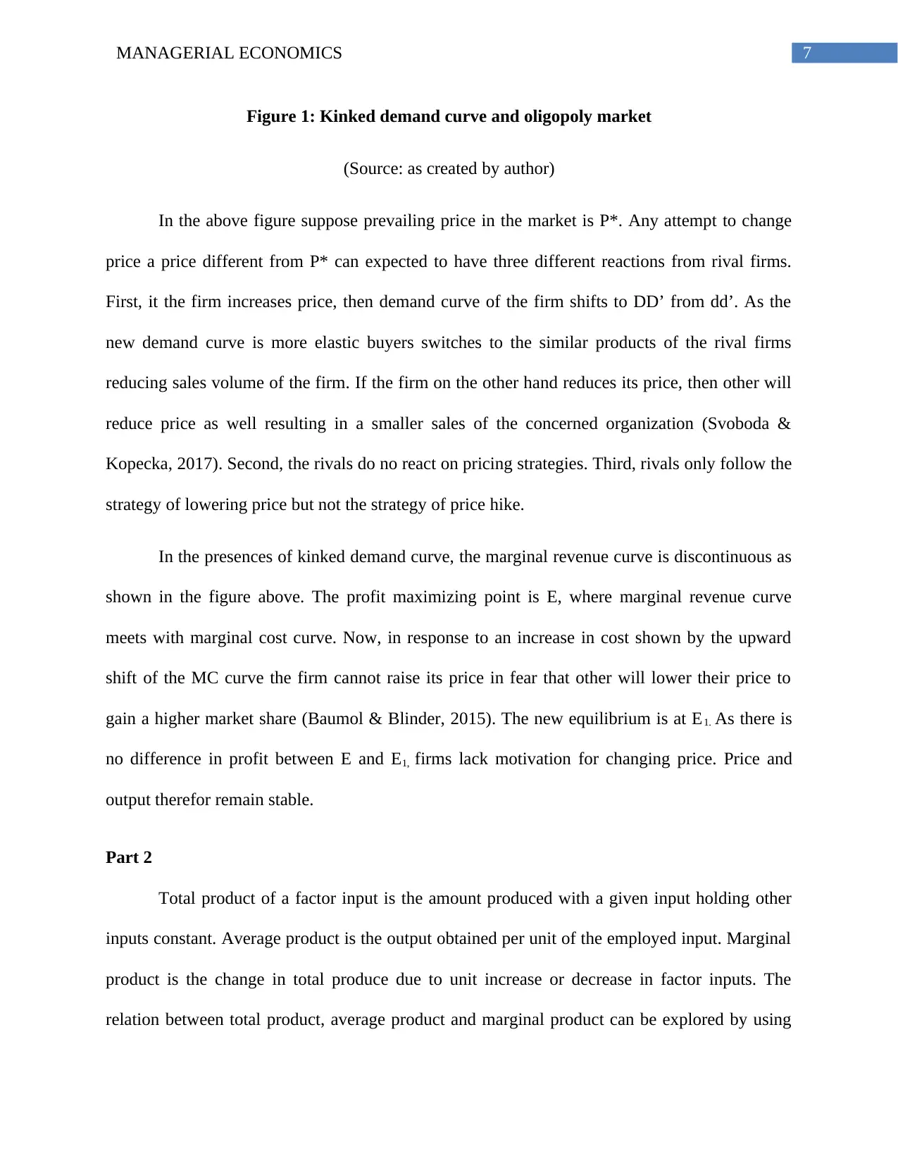
Figure 1: Kinked demand curve and oligopoly market
(Source: as created by author)
In the above figure suppose prevailing price in the market is P*. Any attempt to change
price a price different from P* can expected to have three different reactions from rival firms.
First, it the firm increases price, then demand curve of the firm shifts to DD’ from dd’. As the
new demand curve is more elastic buyers switches to the similar products of the rival firms
reducing sales volume of the firm. If the firm on the other hand reduces its price, then other will
reduce price as well resulting in a smaller sales of the concerned organization (Svoboda &
Kopecka, 2017). Second, the rivals do no react on pricing strategies. Third, rivals only follow the
strategy of lowering price but not the strategy of price hike.
In the presences of kinked demand curve, the marginal revenue curve is discontinuous as
shown in the figure above. The profit maximizing point is E, where marginal revenue curve
meets with marginal cost curve. Now, in response to an increase in cost shown by the upward
shift of the MC curve the firm cannot raise its price in fear that other will lower their price to
gain a higher market share (Baumol & Blinder, 2015). The new equilibrium is at E1. As there is
no difference in profit between E and E1, firms lack motivation for changing price. Price and
output therefor remain stable.
Part 2
Total product of a factor input is the amount produced with a given input holding other
inputs constant. Average product is the output obtained per unit of the employed input. Marginal
product is the change in total produce due to unit increase or decrease in factor inputs. The
relation between total product, average product and marginal product can be explored by using

8MANAGERIAL ECONOMICS
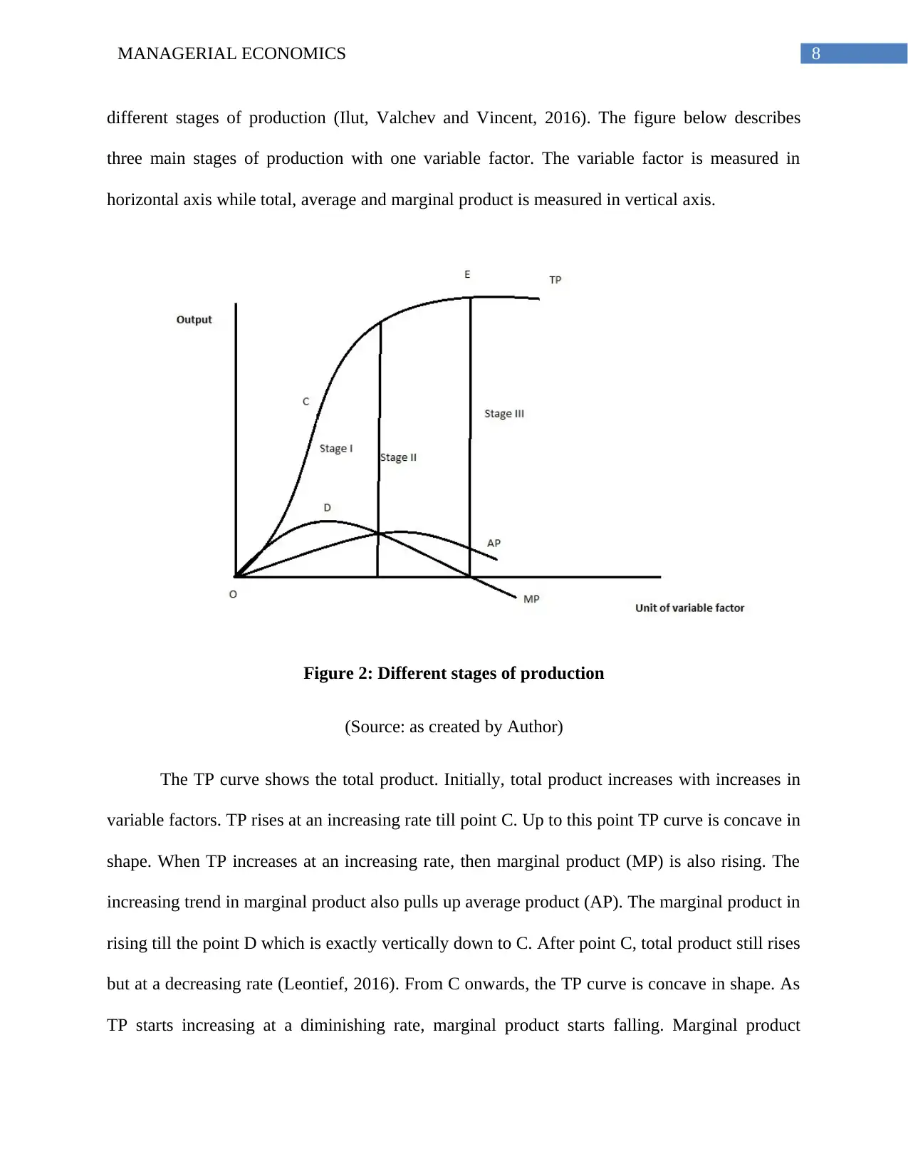
different stages of production (Ilut, Valchev and Vincent, 2016). The figure below describes
three main stages of production with one variable factor. The variable factor is measured in
horizontal axis while total, average and marginal product is measured in vertical axis.
Figure 2: Different stages of production
(Source: as created by Author)
The TP curve shows the total product. Initially, total product increases with increases in
variable factors. TP rises at an increasing rate till point C. Up to this point TP curve is concave in
shape. When TP increases at an increasing rate, then marginal product (MP) is also rising. The
increasing trend in marginal product also pulls up average product (AP). The marginal product in
rising till the point D which is exactly vertically down to C. After point C, total product still rises
but at a decreasing rate (Leontief, 2016). From C onwards, the TP curve is concave in shape. As
TP starts increasing at a diminishing rate, marginal product starts falling. Marginal product

9MANAGERIAL ECONOMICS
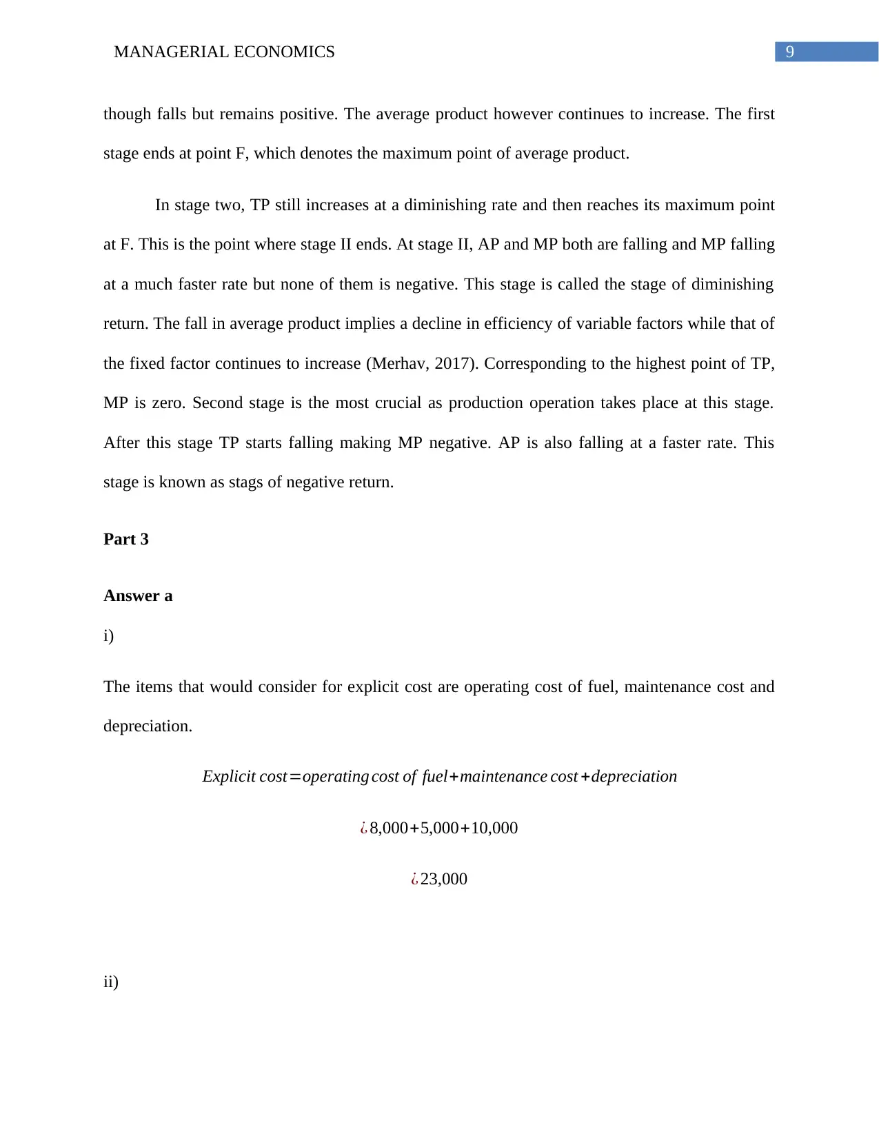
though falls but remains positive. The average product however continues to increase. The first
stage ends at point F, which denotes the maximum point of average product.
In stage two, TP still increases at a diminishing rate and then reaches its maximum point
at F. This is the point where stage II ends. At stage II, AP and MP both are falling and MP falling
at a much faster rate but none of them is negative. This stage is called the stage of diminishing
return. The fall in average product implies a decline in efficiency of variable factors while that of
the fixed factor continues to increase (Merhav, 2017). Corresponding to the highest point of TP,
MP is zero. Second stage is the most crucial as production operation takes place at this stage.
After this stage TP starts falling making MP negative. AP is also falling at a faster rate. This
stage is known as stags of negative return.
Part 3
Answer a
i)
The items that would consider for explicit cost are operating cost of fuel, maintenance cost and
depreciation.
Explicit cost=operating cost of fuel+maintenance cost +depreciation
¿ 8,000+5,000+10,000
¿ 23,000
ii)

10MANAGERIAL ECONOMICS
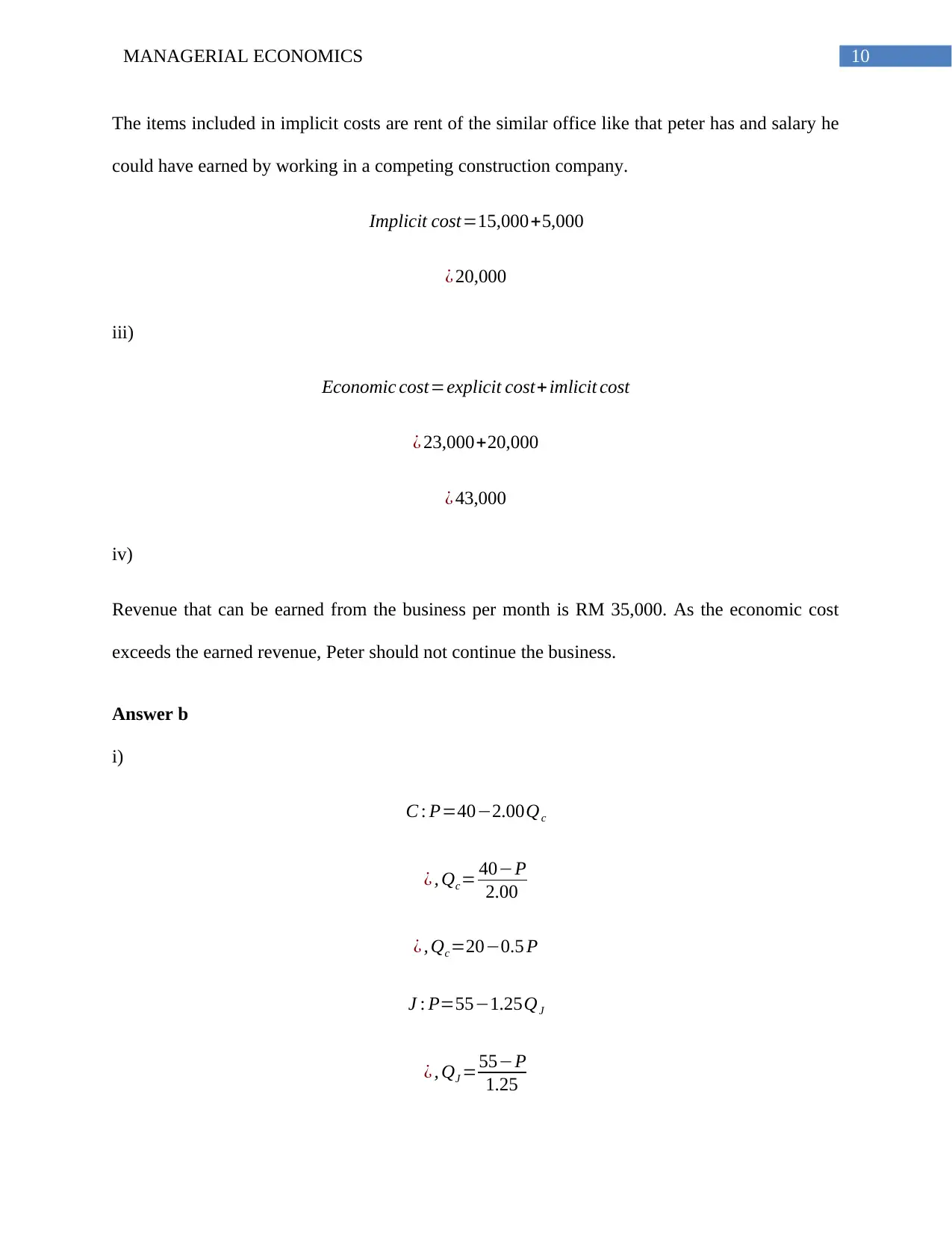
The items included in implicit costs are rent of the similar office like that peter has and salary he
could have earned by working in a competing construction company.
Implicit cost=15,000+5,000
¿ 20,000
iii)
Economic cost=explicit cost+ imlicit cost
¿ 23,000+20,000
¿ 43,000
iv)
Revenue that can be earned from the business per month is RM 35,000. As the economic cost
exceeds the earned revenue, Peter should not continue the business.
Answer b
i)
C : P=40−2.00Qc
¿ , Qc= 40−P
2.00
¿ , Qc=20−0.5 P
J : P=55−1.25QJ
¿ , QJ =55−P
1.25

11MANAGERIAL ECONOMICS
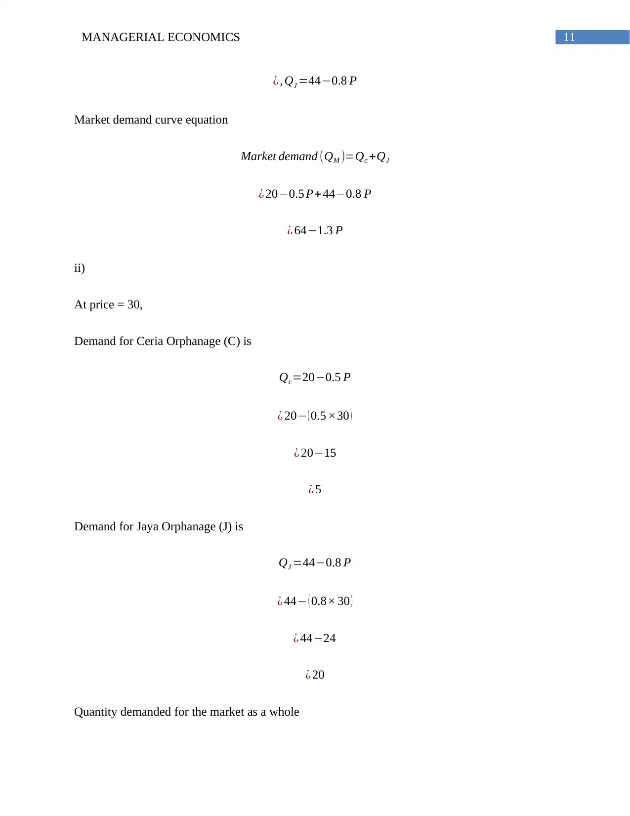
¿ , QJ =44−0.8 P
Market demand curve equation
Market demand (QM )=Qc +QJ
¿ 20−0.5 P+ 44−0.8 P
¿ 64−1.3 P
ii)
At price = 30,
Demand for Ceria Orphanage (C) is
Qc=20−0.5 P
¿ 20− ( 0.5 ×30 )
¿ 20−15
¿ 5
Demand for Jaya Orphanage (J) is
QJ =44−0.8 P
¿ 44− ( 0.8× 30 )
¿ 44−24
¿ 20
Quantity demanded for the market as a whole