Managerial Economics Assignment: Investment, Demand, and Costs

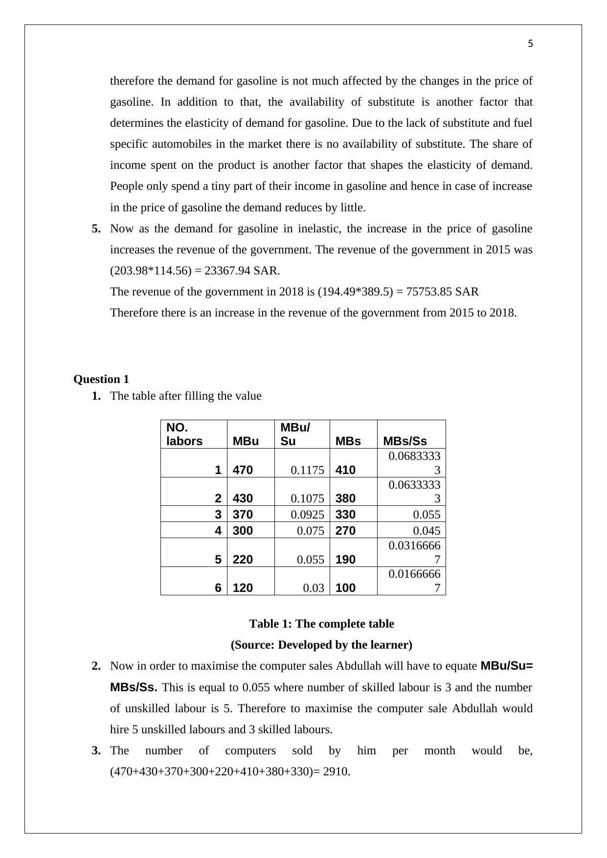
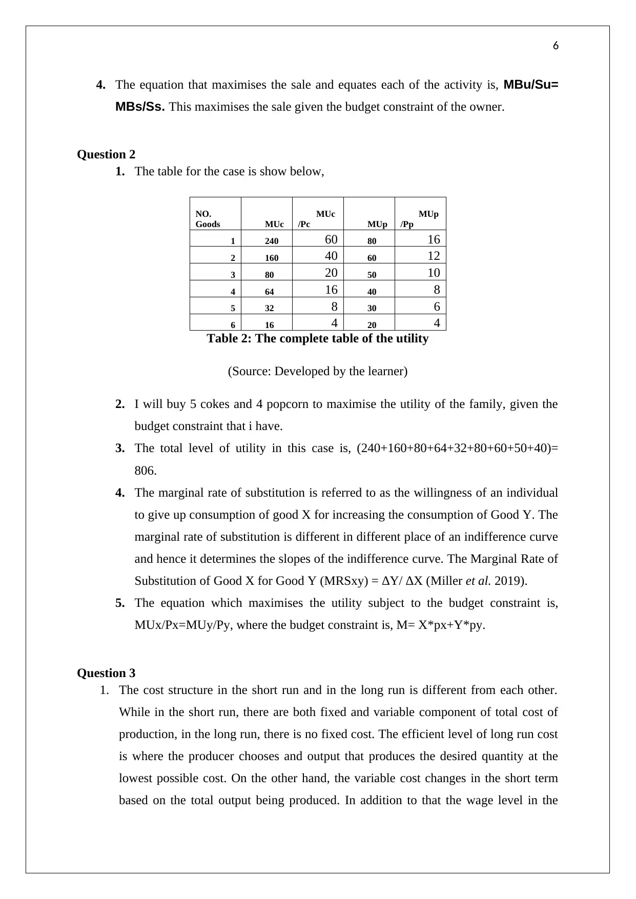
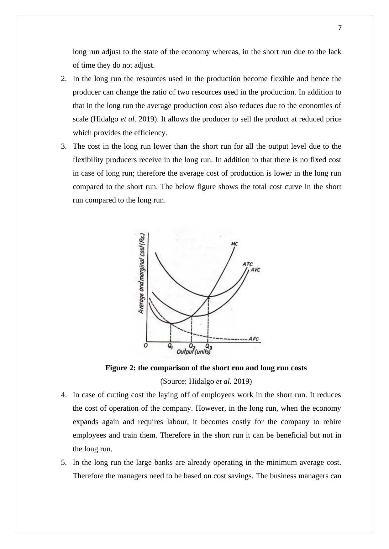
This assignment solution addresses key concepts in managerial economics through a series of questions. The first question analyzes an investment in the textile industry, calculating present value, economic and accounting profits, and the impact of inflation. The second question examines demand...Read More

1
MANAGERIAL ECONOMICS

2
Contents
Question 1..................................................................................................................................3
Question 2..................................................................................................................................3
Question 3..................................................................................................................................4
Question 1..................................................................................................................................5
Question 2..................................................................................................................................6
Question 3..................................................................................................................................6
Reference....................................................................................................................................8

3
Question 1
1. The explicit cost of the industry is the salaries provided to the workers and the
implicit costs are the opportunity cost of investing this money in other industries.
2. The NPV= F / [ (1 + i)^n ] => 10/[(1+0.06)^3]= 8.39 Million SAR. Therefore, it can
be sold in any price more than the NPV in order to earn profit.
3. The industry is economically profitable as the Net Present value of the industry is less
than the expected return from the investment.
4. The difference between the economic and accounting profit is mainly due to the
incorporation of opportunity cost. The economic profit in this case is, (12-8.39)= 3.61
Million SAR. On the other hand the accounting profit is, (12-10)= 2 Million SAR.
Therefore the difference is 1.61 Million SAR.
5. The high unexpected inflation rate in the economy would increase the interest rates in
other industries and hence the present value of the industry will reduce.
Question 2
1. The relationship of price with quantity demanded is negative and with quantity
supplied is positive. This is consistent with the law of demand as the demand
increases when the price falls and supply increases when the price increases.
2. The coefficient of M, in the equation of quantity demand is positive. That means, with
increase in the income, the demand for the date increases. In case of an inferior good
the coefficient of M would have been negative. However, the coefficient of M is 0.01
which means that for 1 unit increase in the income the demand for date increases by
0.01 units.
3. The determinants of demand as per the demand functions are, Price of dates, Income,
price of related goods and expected price of dates.
4. According to the demand function, the coefficient of price of related product is
positive. That means if the price of related product which in this case is chocolate
increases, the demand for date increases. Therefore, here the cross price elasticity of
demand for date is positive and hence the related product (Chocolate) is substitute to
date.

4
5. As there is no change in the price of dates, the increase in the quantity demanded by
20 tons is a shift in the demand curve. In this case the demand curve shifts to the right
side. Now, the increase in the quantity demand will not influence the quantity supply
directly and hence the supply curve will remain the same. Therefore, the new demand
and the old supply curve will increase the equilibrium price and the quantity in the
date market.
Figure 1: The rightward shift in the demand curve
(Source: Hidalgo et al. 2019)
Question 3
1. The price elasticity of demand for gasoline over the time period is,
((194.49-203.98)/203.98)/((389.5-114.56)/114.56)= -0.019 Approx
2. The demand for gasoline is inelastic as the change in the demand corresponding to a
corresponding change in the price is more than 1. That means the percentage
reduction in demand for gasoline is less than the percentage increase in the price
level.
3. The gasoline and automobile are complementary to each other that means used
together. Now if the gasoline price increases the maintenance cost of automobile will
also increase and hence the demand for automobile will reduce. If the price of
gasoline increases the quantity demanded of automobile will reduce. Therefore the
cross price elasticity of demand for automobile is negative. This is also consistent
with the fact that these two goods are complementary to each other.
4. The price elasticity of demand is affected by a number of factors that includes the
nature of the commodity. Gasoline is only fuel which can be used in the automobile;

5
therefore the demand for gasoline is not much affected by the changes in the price of
gasoline. In addition to that, the availability of substitute is another factor that
determines the elasticity of demand for gasoline. Due to the lack of substitute and fuel
specific automobiles in the market there is no availability of substitute. The share of
income spent on the product is another factor that shapes the elasticity of demand.
People only spend a tiny part of their income in gasoline and hence in case of increase
in the price of gasoline the demand reduces by little.
5. Now as the demand for gasoline in inelastic, the increase in the price of gasoline
increases the revenue of the government. The revenue of the government in 2015 was
(203.98*114.56) = 23367.94 SAR.
The revenue of the government in 2018 is (194.49*389.5) = 75753.85 SAR
Therefore there is an increase in the revenue of the government from 2015 to 2018.
Question 1
1. The table after filling the value
NO.
labors MBu
MBu/
Su MBs MBs/Ss
1 470 0.1175 410
0.0683333
3
2 430 0.1075 380
0.0633333
3
3 370 0.0925 330 0.055
4 300 0.075 270 0.045
5 220 0.055 190
0.0316666
7
6 120 0.03 100
0.0166666
7
Table 1: The complete table
(Source: Developed by the learner)
2. Now in order to maximise the computer sales Abdullah will have to equate MBu/Su=
MBs/Ss. This is equal to 0.055 where number of skilled labour is 3 and the number
of unskilled labour is 5. Therefore to maximise the computer sale Abdullah would
hire 5 unskilled labours and 3 skilled labours.
3. The number of computers sold by him per month would be,
(470+430+370+300+220+410+380+330)= 2910.

6
4. The equation that maximises the sale and equates each of the activity is, MBu/Su=
MBs/Ss. This maximises the sale given the budget constraint of the owner.
Question 2
1. The table for the case is show below,
NO.
Goods MUc
MUc
/Pc MUp
MUp
/Pp
1 240 60 80 16
2 160 40 60 12
3 80 20 50 10
4 64 16 40 8
5 32 8 30 6
6 16 4 20 4
Table 2: The complete table of the utility
(Source: Developed by the learner)
2. I will buy 5 cokes and 4 popcorn to maximise the utility of the family, given the
budget constraint that i have.
3. The total level of utility in this case is, (240+160+80+64+32+80+60+50+40)=
806.
4. The marginal rate of substitution is referred to as the willingness of an individual
to give up consumption of good X for increasing the consumption of Good Y. The
marginal rate of substitution is different in different place of an indifference curve
and hence it determines the slopes of the indifference curve. The Marginal Rate of
Substitution of Good X for Good Y (MRSxy) = ∆Y/ ∆X (Miller et al. 2019).
5. The equation which maximises the utility subject to the budget constraint is,
MUx/Px=MUy/Py, where the budget constraint is, M= X*px+Y*py.
Question 3
1. The cost structure in the short run and in the long run is different from each other.
While in the short run, there are both fixed and variable component of total cost of
production, in the long run, there is no fixed cost. The efficient level of long run cost
is where the producer chooses and output that produces the desired quantity at the
lowest possible cost. On the other hand, the variable cost changes in the short term
based on the total output being produced. In addition to that the wage level in the

7
long run adjust to the state of the economy whereas, in the short run due to the lack
of time they do not adjust.
2. In the long run the resources used in the production become flexible and hence the
producer can change the ratio of two resources used in the production. In addition to
that in the long run the average production cost also reduces due to the economies of
scale (Hidalgo et al. 2019). It allows the producer to sell the product at reduced price
which provides the efficiency.
3. The cost in the long run lower than the short run for all the output level due to the
flexibility producers receive in the long run. In addition to that there is no fixed cost
in case of long run; therefore the average cost of production is lower in the long run
compared to the short run. The below figure shows the total cost curve in the short
run compared to the long run.
Figure 2: the comparison of the short run and long run costs
(Source: Hidalgo et al. 2019)
4. In case of cutting cost the laying off of employees work in the short run. It reduces
the cost of operation of the company. However, in the long run, when the economy
expands again and requires labour, it becomes costly for the company to rehire
employees and train them. Therefore in the short run it can be beneficial but not in
the long run.
5. In the long run the large banks are already operating in the minimum average cost.
Therefore the managers need to be based on cost savings. The business managers can

8
rather increase the productivity of the labours in order to increase the profitability of
the large banks.

9
Reference
Hidalgo, César A., et al. "The principle of relatedness." International conference on complex
systems. Springer, Cham, 2018.
Miller, Joshua B., and Adam Sanjurjo. "A Bridge from Monty Hall to the Hot Hand: The
Principle of Restricted Choice." Journal of Economic Perspectives 33.3 (2019): 144-
62.