Managerial Economics Assignment Solution: Comprehensive Analysis
VerifiedAdded on 2023/04/25
|39
|9292
|77
Homework Assignment
AI Summary
This document presents a complete solution to a managerial economics assignment. Part A addresses topics such as the calculation of financial and economic costs, profit maximization using marginal revenue and marginal cost, the concept of price elasticity of demand and its determinants, price discrimination strategies with examples from the airline industry, and the law of diminishing returns in relation to short-run cost curves. Part B delves into the application of economic principles to real-world scenarios, providing detailed answers to practical questions. The solution includes calculations, explanations, and relevant economic theories to offer a thorough understanding of the subject matter. This comprehensive resource is designed to aid students in their coursework and enhance their grasp of managerial economics principles.
Running head: MANAGERIAL ECONOMICS
Managerial Economics
Name of the Student
Name of the University
Course ID
Managerial Economics
Name of the Student
Name of the University
Course ID
Paraphrase This Document
Need a fresh take? Get an instant paraphrase of this document with our AI Paraphraser
1MANAGERIAL ECONOMICS
Table of Contents
Part A.........................................................................................................................................2
Answer 1................................................................................................................................2
Answer 2................................................................................................................................3
Answer 3................................................................................................................................4
Answer 4................................................................................................................................6
Answer 5................................................................................................................................9
Answer 6..............................................................................................................................14
Answer 7..............................................................................................................................17
Part B........................................................................................................................................21
Answer 1..............................................................................................................................21
Answer 2..............................................................................................................................24
Answer 3..............................................................................................................................27
References................................................................................................................................32
2MANAGERIAL ECONOMICS
Part A
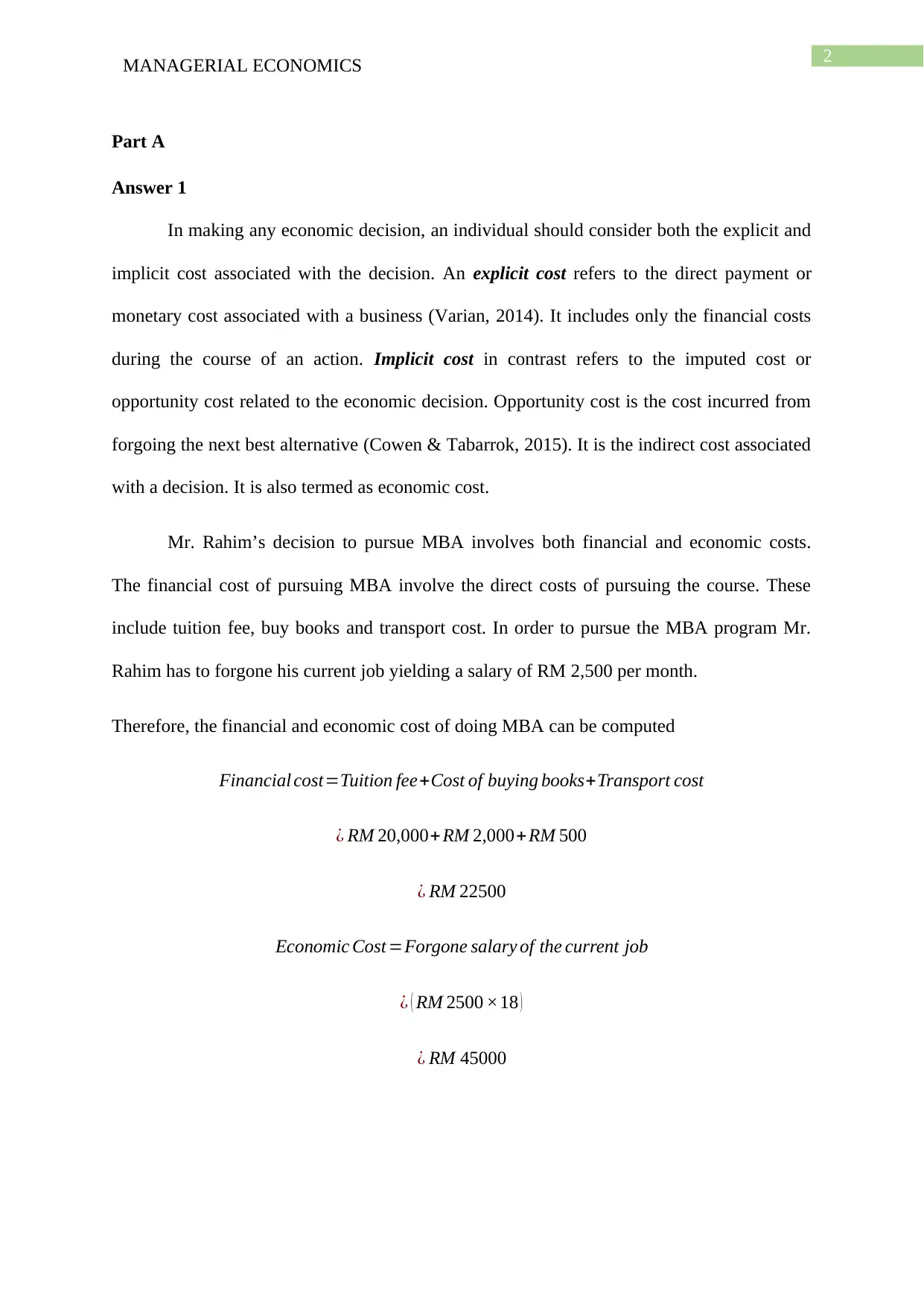
Answer 1
In making any economic decision, an individual should consider both the explicit and
implicit cost associated with the decision. An explicit cost refers to the direct payment or
monetary cost associated with a business (Varian, 2014). It includes only the financial costs
during the course of an action. Implicit cost in contrast refers to the imputed cost or
opportunity cost related to the economic decision. Opportunity cost is the cost incurred from
forgoing the next best alternative (Cowen & Tabarrok, 2015). It is the indirect cost associated
with a decision. It is also termed as economic cost.
Mr. Rahim’s decision to pursue MBA involves both financial and economic costs.
The financial cost of pursuing MBA involve the direct costs of pursuing the course. These
include tuition fee, buy books and transport cost. In order to pursue the MBA program Mr.
Rahim has to forgone his current job yielding a salary of RM 2,500 per month.
Therefore, the financial and economic cost of doing MBA can be computed
Financial cost=Tuition fee+Cost of buying books+Transport cost
¿ RM 20,000+RM 2,000+ RM 500
¿ RM 22500
Economic Cost =Forgone salary of the current job
¿ ( RM 2500 ×18 )
¿ RM 45000
Part A
Answer 1
In making any economic decision, an individual should consider both the explicit and
implicit cost associated with the decision. An explicit cost refers to the direct payment or
monetary cost associated with a business (Varian, 2014). It includes only the financial costs
during the course of an action. Implicit cost in contrast refers to the imputed cost or
opportunity cost related to the economic decision. Opportunity cost is the cost incurred from
forgoing the next best alternative (Cowen & Tabarrok, 2015). It is the indirect cost associated
with a decision. It is also termed as economic cost.
Mr. Rahim’s decision to pursue MBA involves both financial and economic costs.
The financial cost of pursuing MBA involve the direct costs of pursuing the course. These
include tuition fee, buy books and transport cost. In order to pursue the MBA program Mr.
Rahim has to forgone his current job yielding a salary of RM 2,500 per month.
Therefore, the financial and economic cost of doing MBA can be computed
Financial cost=Tuition fee+Cost of buying books+Transport cost
¿ RM 20,000+RM 2,000+ RM 500
¿ RM 22500
Economic Cost =Forgone salary of the current job
¿ ( RM 2500 ×18 )
¿ RM 45000
⊘ This is a preview!⊘
Do you want full access?
Subscribe today to unlock all pages.
Trusted by 1+ million students worldwide
3MANAGERIAL ECONOMICS
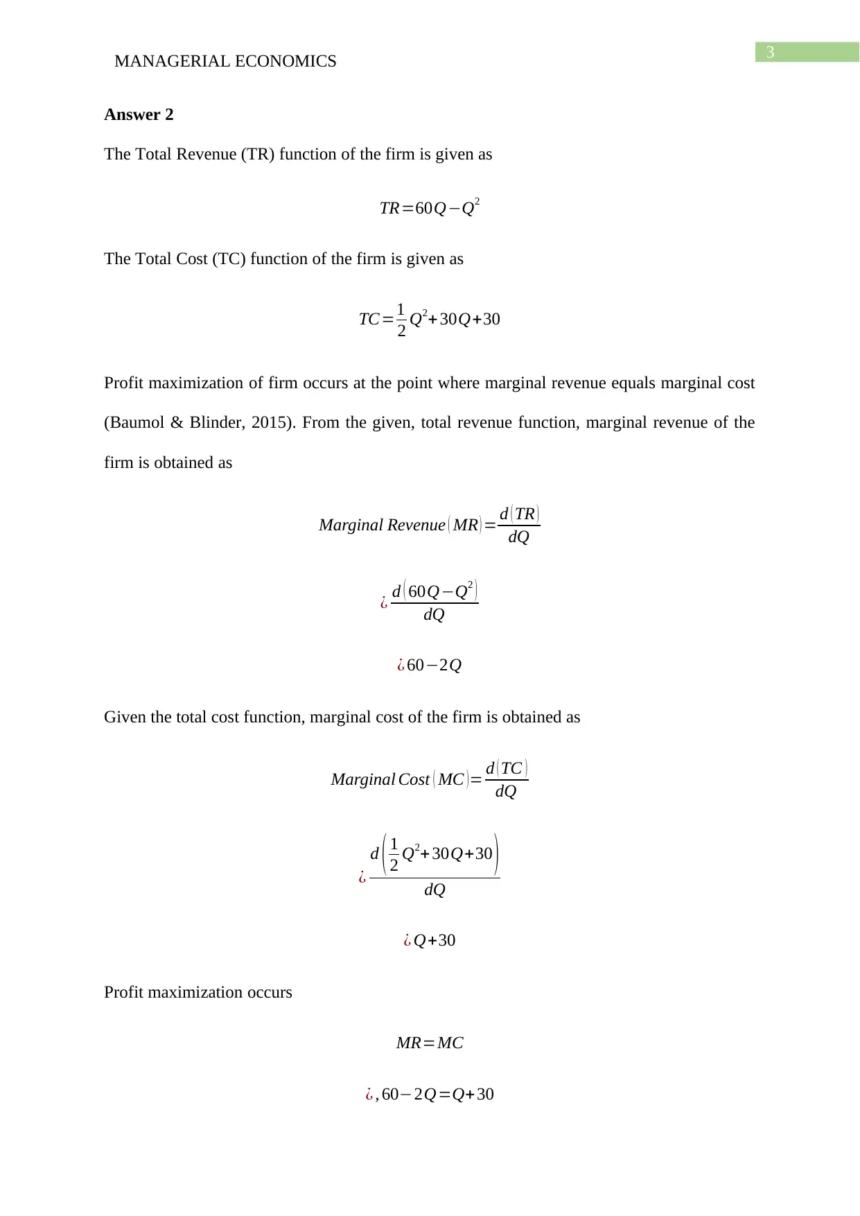
Answer 2
The Total Revenue (TR) function of the firm is given as
TR=60Q−Q2
The Total Cost (TC) function of the firm is given as
TC=1
2 Q2+ 30Q+30
Profit maximization of firm occurs at the point where marginal revenue equals marginal cost
(Baumol & Blinder, 2015). From the given, total revenue function, marginal revenue of the
firm is obtained as
Marginal Revenue ( MR ) = d ( TR )
dQ
¿ d ( 60Q−Q2 )
dQ
¿ 60−2Q
Given the total cost function, marginal cost of the firm is obtained as
Marginal Cost ( MC ) = d ( TC )
dQ
¿
d ( 1
2 Q2+ 30Q+30 )
dQ
¿ Q+30
Profit maximization occurs
MR=MC
¿ , 60−2Q=Q+30
Paraphrase This Document
Need a fresh take? Get an instant paraphrase of this document with our AI Paraphraser
4MANAGERIAL ECONOMICS
¿ , 2Q+Q=60−30
¿ , 3 Q=30
¿ , Q= 30
3
¿ , Q=10
The quantity level that maximizes total profit of the firm is obtained as 10.
Answer 3
Price elasticity of demand
The term price elastic of demand in economic measures the percentage change in
quantity demanded of a commodity in response to a percentage change in price (Whitehead,
2014). Price elasticity of demand actually measures the responsiveness of demand for a
change in price.
It is measured by computing the percentage change in quantity demanded with respect to
certain percentage change in price.
Price elasticity of demand= Percentage change∈quantity demanded
Percentage chamge∈ price
Determinants of demand
The first primary determinant of demand is price of the product. Given all the factors,
an increase in price lowers demand and vice-versa. Except price, several factors influence
demand of the product. Some of the factors determining demand of a product are discussed
below.
5MANAGERIAL ECONOMICS
Income
In case of a normal good, income has a positive relation with demand. That is as
income increases, ceteris paribus demand for a good or service increases and vice-versa
(Kreps, 2019). Goods for which this does not hold, that is demand reduces with increase in
income are termed as inferior good.
Taste and preferences
Tastes and preferences capture personal like or dislike of buyers of various goods and
services. Tastes and preferences are again influenced by religious belief, advertising, culture,
government reports, promotions, campaign and such other factors. Increasing preference for a
good increases demand and vice-versa.
Price of related good
Related goods of particular goods referred as either substitutes or complements of the
good. When price of a substitute good increases, demand for the concerned good increases as
consumers look for relatively cheaper substitutes (Bade & Parkin, 2015). For example, tea
and coffee. When price of a complementary good increases, demand for the particular good
decreases as consumers to reduce demand for the good along with its complementary good.
For example car and petrol.
Number of consumers/population
The effect of number of buyers on demand for a product varies depending on interest
of changing demographics and associated tastes and preferences.
Future expectation
Buyers’ expectation that price of a good or service will increase in future; encourage
buyers to increase their current demand (McKenzie & Lee, 2016).
⊘ This is a preview!⊘
Do you want full access?
Subscribe today to unlock all pages.
Trusted by 1+ million students worldwide
6MANAGERIAL ECONOMICS
Optimal Price ( P )= Marginal Cost ( MC )
(1+ 1
Ed )
¿ 200
1− 1
3
¿ 200
2
3
¿ 200 × 3
2
¿ RM 300
Answer 4
Price Discrimination:
Price discrimination refers to the producers’ practices of charging different prices to
different consumers for the same good or service. Under free market, total surplus is divided
between consumers and producers. When producers have sufficient market power then they
try to increase their surplus by practicing price discrimination (Paczkowski, 2019). There are
three types of price discrimination: first degree price discrimination, second degree price
discrimination and third degree price discrimination.
First degree price discrimination: Seller charges highest possible price for each unit of
good. In this case, there is no consumer surplus for the buyers. There is no deadweight loss in
the case of first-degree price discrimination. Social welfare is increased in this case even after
complete extraction of consumers’ surplus. (Pepall, Richards & Norman, 2014)
Second Degree price discrimination: Under second degree price discrimination, firm knows
that different consumers in the market has different demand functions however the demand
Paraphrase This Document
Need a fresh take? Get an instant paraphrase of this document with our AI Paraphraser
7MANAGERIAL ECONOMICS
function of a particular consumer is not known. Firm here offers a menu price for different
packages. Options are designed in such a way consumers can self-select by choosing suitable
package for themselves. Unlike first-degree price discrimination, firms by practicing second-
degree price discrimination cannot capture all consumer surplus.
Third Degree price discrimination: In this case, seller charges according to the elasticity of
demand among different group of buyers. Price discriminator will separate buyers in different
groups having different elasticity of demand (Waldman & Jensen, 2016). Now, the seller will
charge lower price for highly demand elastic market and higher price for lower demand
elastic market. Third degree price discrimination cannot increase the social welfare.
Conditions for Effective price discrimination:
To discriminate price effectively, seller need to identify the demands of the buyers or the
group of the buyers. Conditions for effective price discrimination are the following:
Immovability of buyers: In order the make price discrimination effective, sellers should
ensure that the buyers are not able to switch from one market to another market. That means
buyers cannot move from high price market to low price market (Gillespie, 2016). Markets
could be separated depending on the following factors:
Time: Different prices are charged in different times of a day or week or month.
Age: Prices are different for different age group. Example, due to reservation for old- age
people, they pay less than other people do.
Region: Transportation cost changes the price of same good. Where the transportation cost is
high, prices are higher in that place and vice versa.
Status: Prices can vary for the status or designation of the buyer. For an example, entry fee or
the charges in a club is different for the club members and non-members.
8MANAGERIAL ECONOMICS
Different elasticity of demand: Price elasticity of demand should be different for different
markets. Price inelastic demand one market enables the market to charge more price in the
market and less in other market (Currie, Peel & Peters, 2016). Different demand enables the
market to charge different price. In the inelastic demand market price is higher than the
elastic market.
Except the above two conditions there are some conditions which are also important
in the process of price discrimination. To discriminate price, firms need market power to
charge above marginal cost. Consumers need to be heterogeneous and resealing of products
needs to be banned or costly.
Price discrimination in the airline industry
In the airline industry, price discrimination is a common phenomenon. Passengers
pays different prices for the same flight and same services in the airline industry. Ticket fare
varies depending on time of booking the tickets, facilities associated with seat, seasons and
other attributes (Cattaneo et al., 2016). The conditions that make the price dissemination
possible in the airline industry are explained below.
1. In the airline industry, the source of market power is the barriers that have been
raised by the scale of economies and sunk cost to discriminate price.
2. They occupy the different schedules of flight. To do so, they offer different routes.
This helps them to differentiate among customers. For example, carriers, which
have too many connections to offer for west coast, make itself different from other
carrier, which flies to the east coast only (Bergantino & Capozza, 2015). Both of
them offer their ticket for sale for Boston-Miami route.
3. Different consumers have different elasticity of demand.
⊘ This is a preview!⊘
Do you want full access?
Subscribe today to unlock all pages.
Trusted by 1+ million students worldwide
9MANAGERIAL ECONOMICS
The airline industry does some common price discrimination, which are described as
below:
Versions of Ticket: Different versions of tickets are available in the airline industry. Such as,
expensive and flexible tickets enable the customer to reschedule the flight and cheap tickets,
which have restrictions.
Discounts to Large Customers: in the national and international level, some large customers
are likely to sign a contract with the airline companies to get discount (Chakrabarty & Kutlu,
2014). Such as, a firm’s employees get discounts on tickets. In this case, different groups of
customers pay different prices.
Frequent Flyers: in this programme, the flyers, which take the flights frequently, get
member points for every confirmed flights. Further, these points are used to get a free flight
as a discount.
Answer 5
Law of Diminishing Returns and Short-Run Cost Curve:
The law of diminishing returns states that increase in the quantity of an input other
things remaining same, the total productivity will increase at decreasing rate. In other words,
increase in the quantity of input other things remaining same; the marginal physical
productivity of the input will fall (Allen et al., 2013). There are certain assumptions, which
are described as follows:
The state of technology remains constant.
Only one input can be changed and other inputs will remain same.
The law is not applicable in case of the production where the inputs are proportionally
required (Shepherd, 2015).
Only physical inputs and outputs are considered.
Paraphrase This Document
Need a fresh take? Get an instant paraphrase of this document with our AI Paraphraser
10MANAGERIAL ECONOMICS
Cost
Quantity
Fixed Cost
Variable Cost
Total Cost
Cost
Quantity
Marginal Cost
Average Total Cost
Average Variable Cost
Average Fixed
Cost
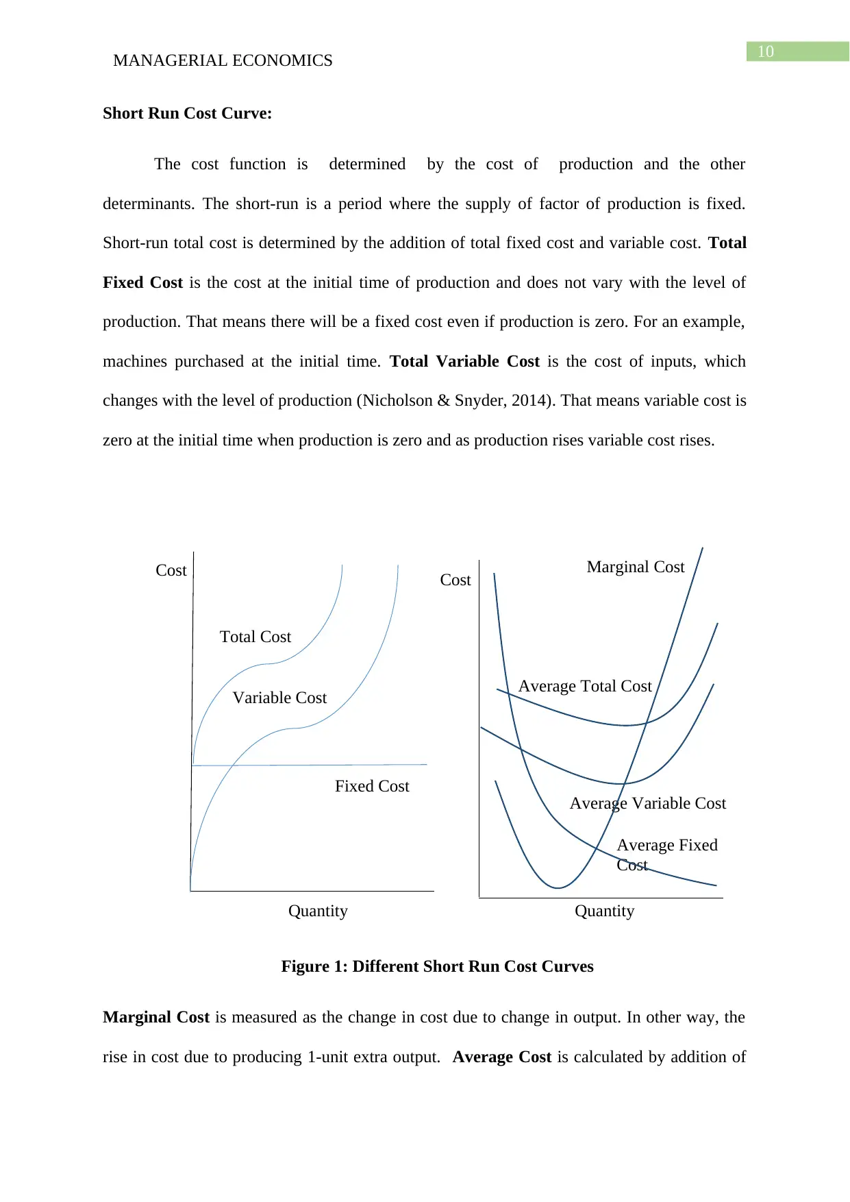
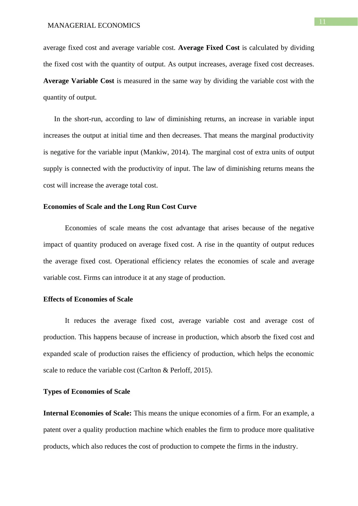
Short Run Cost Curve:
The cost function is determined by the cost of production and the other
determinants. The short-run is a period where the supply of factor of production is fixed.
Short-run total cost is determined by the addition of total fixed cost and variable cost. Total
Fixed Cost is the cost at the initial time of production and does not vary with the level of
production. That means there will be a fixed cost even if production is zero. For an example,
machines purchased at the initial time. Total Variable Cost is the cost of inputs, which
changes with the level of production (Nicholson & Snyder, 2014). That means variable cost is
zero at the initial time when production is zero and as production rises variable cost rises.
Figure 1: Different Short Run Cost Curves
Marginal Cost is measured as the change in cost due to change in output. In other way, the
rise in cost due to producing 1-unit extra output. Average Cost is calculated by addition of
Cost
Quantity
Fixed Cost
Variable Cost
Total Cost
Cost
Quantity
Marginal Cost
Average Total Cost
Average Variable Cost
Average Fixed
Cost
Short Run Cost Curve:
The cost function is determined by the cost of production and the other
determinants. The short-run is a period where the supply of factor of production is fixed.
Short-run total cost is determined by the addition of total fixed cost and variable cost. Total
Fixed Cost is the cost at the initial time of production and does not vary with the level of
production. That means there will be a fixed cost even if production is zero. For an example,
machines purchased at the initial time. Total Variable Cost is the cost of inputs, which
changes with the level of production (Nicholson & Snyder, 2014). That means variable cost is
zero at the initial time when production is zero and as production rises variable cost rises.
Figure 1: Different Short Run Cost Curves
Marginal Cost is measured as the change in cost due to change in output. In other way, the
rise in cost due to producing 1-unit extra output. Average Cost is calculated by addition of
11MANAGERIAL ECONOMICS
average fixed cost and average variable cost. Average Fixed Cost is calculated by dividing
the fixed cost with the quantity of output. As output increases, average fixed cost decreases.
Average Variable Cost is measured in the same way by dividing the variable cost with the
quantity of output.
In the short-run, according to law of diminishing returns, an increase in variable input
increases the output at initial time and then decreases. That means the marginal productivity
is negative for the variable input (Mankiw, 2014). The marginal cost of extra units of output
supply is connected with the productivity of input. The law of diminishing returns means the
cost will increase the average total cost.
Economies of Scale and the Long Run Cost Curve
Economies of scale means the cost advantage that arises because of the negative
impact of quantity produced on average fixed cost. A rise in the quantity of output reduces
the average fixed cost. Operational efficiency relates the economies of scale and average
variable cost. Firms can introduce it at any stage of production.
Effects of Economies of Scale
It reduces the average fixed cost, average variable cost and average cost of
production. This happens because of increase in production, which absorb the fixed cost and
expanded scale of production raises the efficiency of production, which helps the economic
scale to reduce the variable cost (Carlton & Perloff, 2015).
Types of Economies of Scale
Internal Economies of Scale: This means the unique economies of a firm. For an example, a
patent over a quality production machine which enables the firm to produce more qualitative
products, which also reduces the cost of production to compete the firms in the industry.
⊘ This is a preview!⊘
Do you want full access?
Subscribe today to unlock all pages.
Trusted by 1+ million students worldwide
1 out of 39
Related Documents


Your All-in-One AI-Powered Toolkit for Academic Success.
+13062052269
info@desklib.com
Available 24*7 on WhatsApp / Email
![[object Object]](/_next/static/media/star-bottom.7253800d.svg)
Unlock your academic potential
Copyright © 2020–2026 A2Z Services. All Rights Reserved. Developed and managed by ZUCOL.