Analyzing Demand for Burger King's Combination 1 Meal

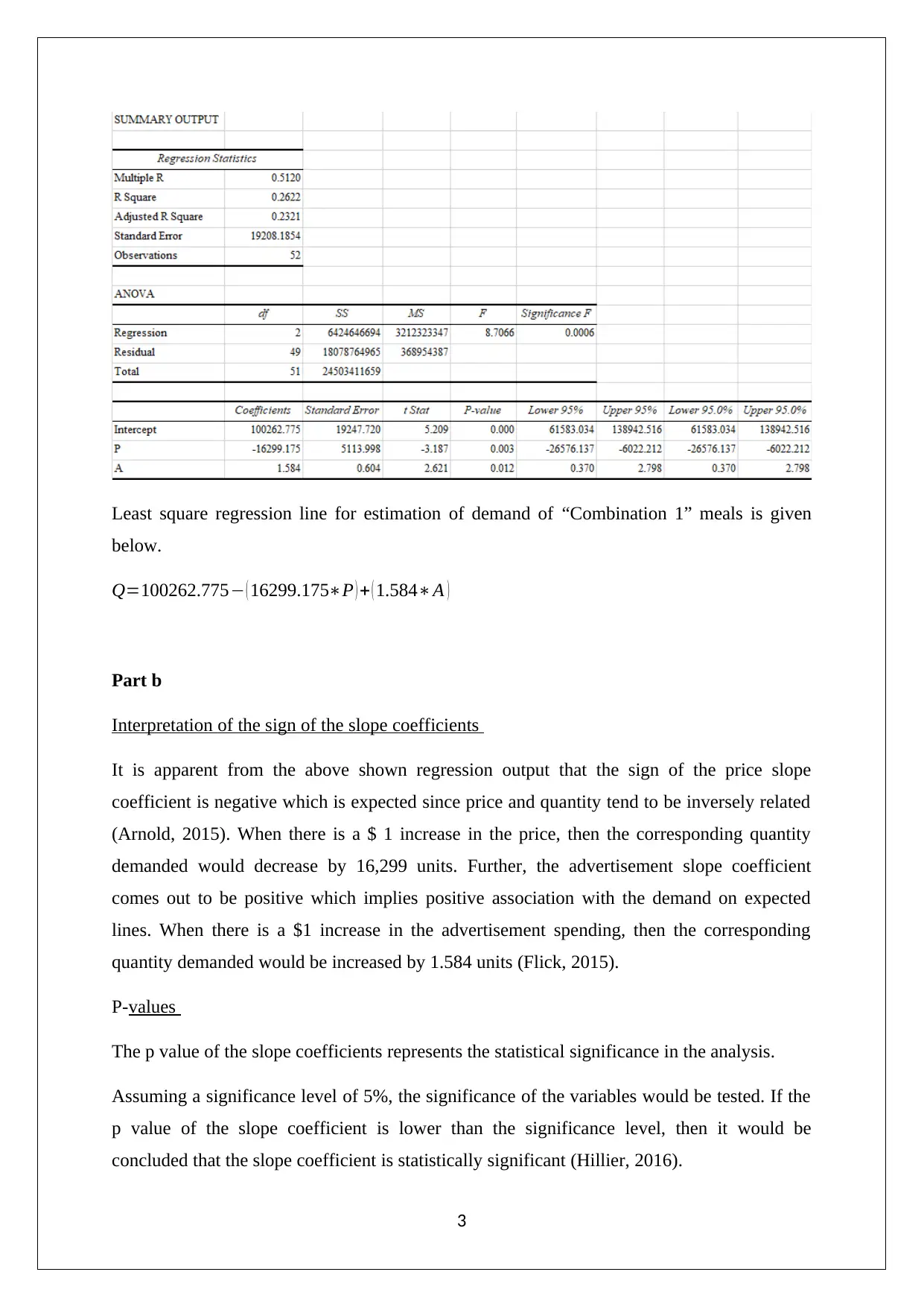
This project analyzes the demand for Burger King's 'Combination 1' meal, based on data provided by the client. The analysis, performed by PWC, focuses on the functional form of the demand function, employing regression analysis to assess the impact of price and advertising expenditure on sales. The report interprets the slope coefficients, assesses their statistical significance using p-values, and calculates the coefficient of determination (R-squared) to evaluate the model's goodness of fit. Furthermore, the project explores factors to improve demand estimation, computes own-price and advertising elasticities, and provides sales forecasts under different price and advertising scenarios. Finally, the project determines the inverse demand price function and calculates the price required to achieve a specific sales volume with a given advertising expenditure. The findings suggest a slightly inelastic demand for the meal and a low advertising elasticity, highlighting the need for additional variables and a larger sample size to improve the model's predictive power.

MANAGERIAL ECONOMICS
STUDENT ID:
[Pick the date]

INTRODUCTION
In the given scenario, PWC has been hired by an client who owns two Atlanta based Burger
King restaurants. The client is operating in a competitive environment as there are
considerable options available to the potential customers. The client wants PWC to study the
demand of the “Combination 1” meal. In order to assist, data has been provided with regards
to sale of “Combination 1” along with the price and advertisement information for each week
in 1998. The objective of this report is to highlight the functional form of demand function
for “Combination 1” meal besides highlighting measures for improvement in demand
estimation. Also, the elasticity of “Combination 1” meal consumption has been computed
with respect to price and advertising spend.
ANALYSIS
Part a
Description of variables
Dependent variable Independent variable
Q = Total number of Combination 1
meals sold
P=¿ Average price charged for Combination 1 meals
A=¿ Dollar amount spent on newspaper ads each week
Linear functional form for the demand for the Combination 1 meals is highlighted below.
Q=a+bP+ cA
Regression model
2

Least square regression line for estimation of demand of “Combination 1” meals is given
below.
Q=100262.775− ( 16299.175∗P ) + ( 1.584∗A )
Part b
Interpretation of the sign of the slope coefficients
It is apparent from the above shown regression output that the sign of the price slope
coefficient is negative which is expected since price and quantity tend to be inversely related
(Arnold, 2015). When there is a $ 1 increase in the price, then the corresponding quantity
demanded would decrease by 16,299 units. Further, the advertisement slope coefficient
comes out to be positive which implies positive association with the demand on expected
lines. When there is a $1 increase in the advertisement spending, then the corresponding
quantity demanded would be increased by 1.584 units (Flick, 2015).
P-values
The p value of the slope coefficients represents the statistical significance in the analysis.
Assuming a significance level of 5%, the significance of the variables would be tested. If the
p value of the slope coefficient is lower than the significance level, then it would be
concluded that the slope coefficient is statistically significant (Hillier, 2016).
3

 For Price (P)
The p value = 0.003
Significance level = 0.05
Observation: p value << significance level
The p value is lower than significance level and hence, it can be said that the slope coefficient
of ‘Price’ is significant.
 For Advertisement (A)
The p value = 0.012
Significance level = 0.05
Observation: p value << significance level
The p value is lower than significance level and hence, it can be said that the slope coefficient
of ‘Advertisement’ is significant.
Coefficient of determination (R2)
From the regression model, it can be seen that the R square value comes out to be 0.2622.
This value implies that only 26.22% variation in the quantity demanded would be jointly
explained by corresponding variation in the price and advertisement variables. Significantly
large portion of the variation is explained by other explanatory variables. Despite this, the
model is a good fit considering that both slopes are significant. Additional predictor variables
need to be added to the model ot improve predictive ability (Eriksson & Kovalainen, 2015).
Part c
The factors that can be used to improve the estimation demand are highlighted as follows
(Flick, 2015).
 Increase the sample size as higher number of weekly data sets would improve the
accuracy of the regression model
 Include other explanatory variables for the analysis as a sizable portion of variation in the
demand depends on the other explanatory variables such as consumer income,
expenditures, price offered by competitors
4

 Include more competitors in the dataset so that one will get different price charged by the
different competitors in Atlanta suburb
Part d
Own price elasticity and advertising elasticity is computed below.
Average price charged for Combination 1 meal = $3.51
Average dollar amount spent on newspaper ads each week = $10009.58
Quantity demanded for this price and advertisement amount
Q=100262.775− ( 16299.175∗P ) + ( 1.584∗A )
Q=100262.775− ( 16299.175∗3.51 ) + ( 1.584∗10009.58 )
Q=58930.98
Hence, the quantity demanded (total number of Combination 1 meals sold) is 58,931.
 Point Price Elasticity
^E= ^b P
Q
P=3.51
Q=58930.98
^b=−16299.175(slope of price)
Now,
^E= ^b P
Q =−16299.175∗3.51
58930.98 =−0.9704
The demand of Combination 1 meals is slightly inelastic. Further, if there is one percent
increase in the price of Combination 1 meals, the weekly sales would decrease by 0.976
percent assuming the other parameters constant (Thomas & Maurice, 2016).
 Advertising Elasticity
^E= ^c A
Q
5

A=10009.58
Q=58930.98
^c=1.584(slope of advertisement)
Now,
^E= ^c A
Q = 1.584∗10009.58
58930.98 =0.269
From the above, it is evident that advertisement elasticity is 0.269. Hence, a 10 percent
increase in the advertisement spending of Combination 1 meals would increase the weekly
sales only by 2.68 percent assuming the other parameters are constant (Mankiw, 2015).
Part e
Price charged for Combination 1 meal = $4.15
Average dollar amount spent on newspaper ads each week = $18,000
Quantity demanded for the given price and advertisement amount =?
Now,
Least square regression line
Q=100262.775− ( 16299.175∗P ) + ( 1.584∗A )
Q=100262.775− ( 16299.175∗4.15 ) + ( 1.584∗18000 )
Q=61130
Hence, 61,130 Combination 1 meals would be sold when the price is $4.15 and expenditure
incurred on advertisement is $18,000.
Part f
Advertisement expenses by the owner = $18000 per week
Quantity demanded for Combination 1 meals = 50,000
Equation for the inverse demand price =?
6

Here,
Q=100262.775− ( 16299.175∗P ) + ( 1.584∗A )
Q=100262.775− ( 16299.175∗P ) + ( 1.584∗18000 )
Q=−16299.175 P+128771.29
P= 1
−16299.175 { ( Q−128771.29 ) }
P=−0.0000614 Q+7.90047
P=7.90047−0.0000614 Q( Requisite inverse demand price function)
Now,
Price when the quantity demanded is 50,000.
P=7.90047− ( 0.0000614∗50000 ) =$ 4.83
The unit price at which $18000 spending on advertisement generates 50,000 units as sale has
been computed as $4.83.
SUMMARY/CONCLUSION
Based on the above analysis, it is evident that a linear functional form is observed for the
estimation of demand. The actual signs of the slope coefficients confirm with the
expectations and are found to be statistically significant. The predictive ability of thee
regression model is not high and suitable independent variables need to be added coupled
with higher sample size. The own price elasticity is 0.97 nearing unitary elasticity. However,
the advertisement related elasticity is 0.27 and hence significantly lower than 1. Also, for
specific scenarios, the demand for Combination 1 meals has also been estimated using the
regression model.
References
Arnold, A.R. (2015). Microeconomics (9thed.). New York, NY: Cengage Learning.
7

Eriksson, P. & Kovalainen, A. (2015). Quantitative methods in business research (3rded.).
London: Sage Publications.
Flick, U. (2015). Introducing research methodology: A beginner's guide to doing a research
project (4thed.). New York: Sage Publications.
Hillier, F. (2016).Introduction to Operations Research.(6thed.). New York: McGraw Hill
Publications
Mankiw, G. (2015) Microeconomics (6thed.). London: Worth Publishers.
Thomas, C. R., & Maurice, S. C. (2016), Managerial economics: Foundations of business
analysis and strategy (12thed.). New York, NY: McGraw-Hill.
8