Managerial Economics Assignment on Market Structures Analysis

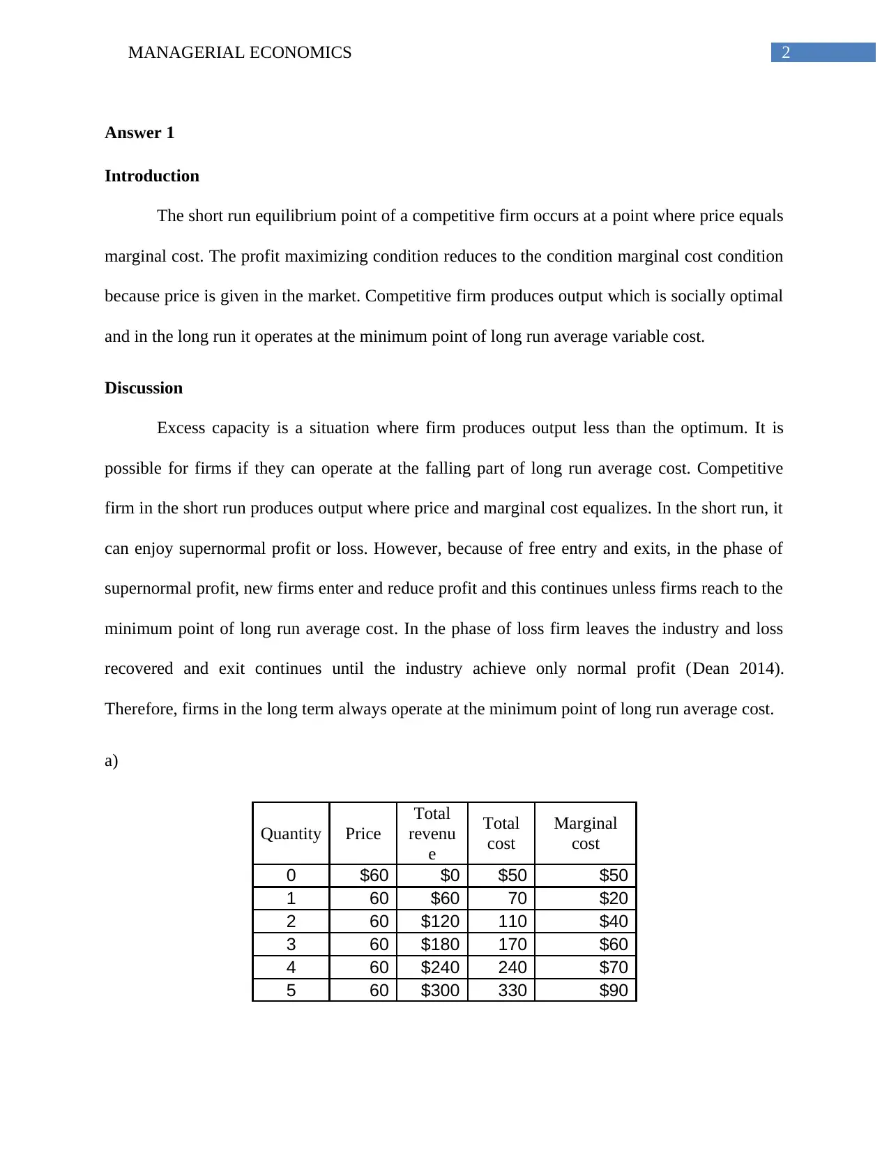
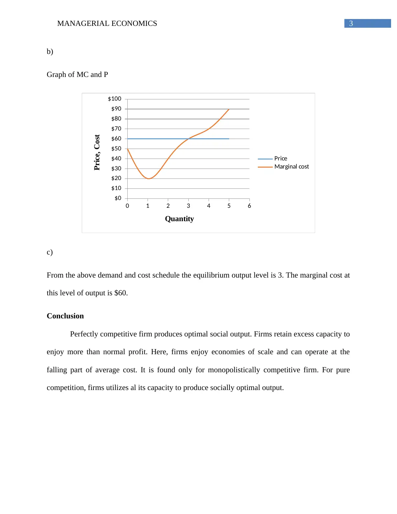
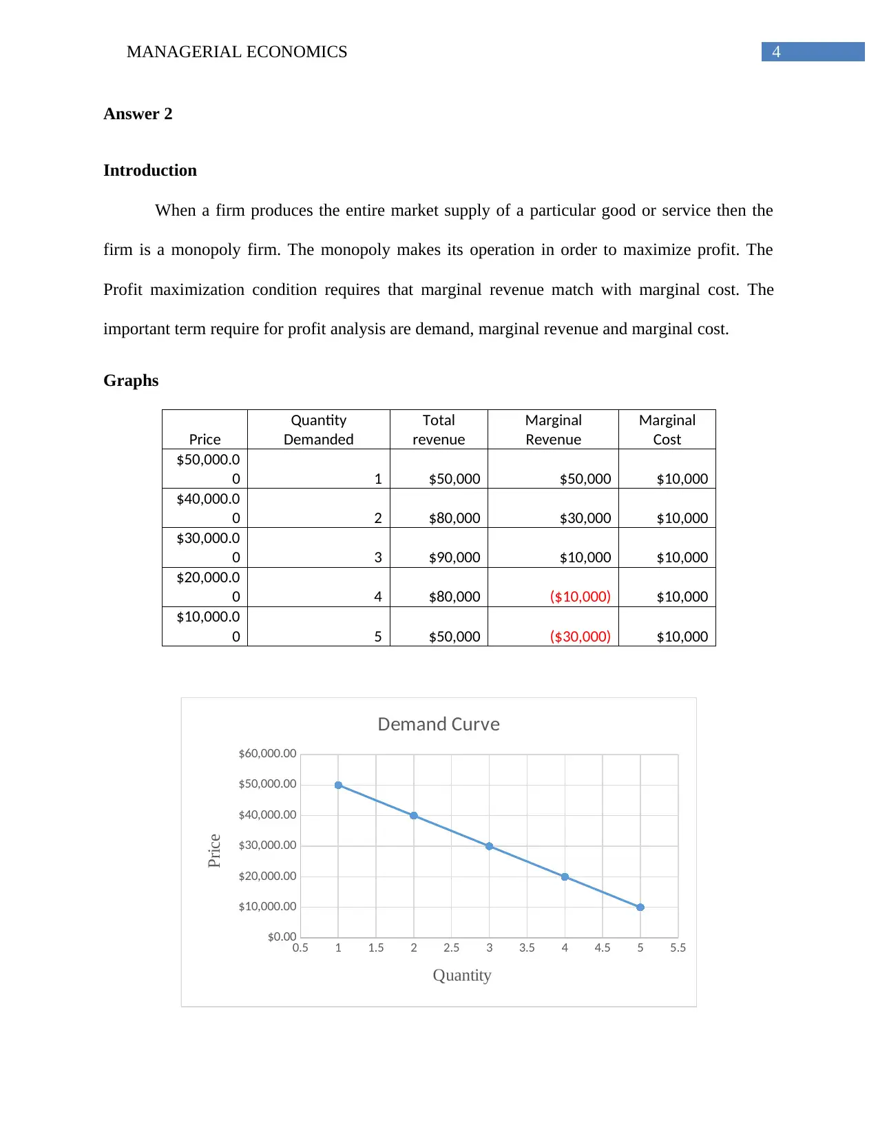
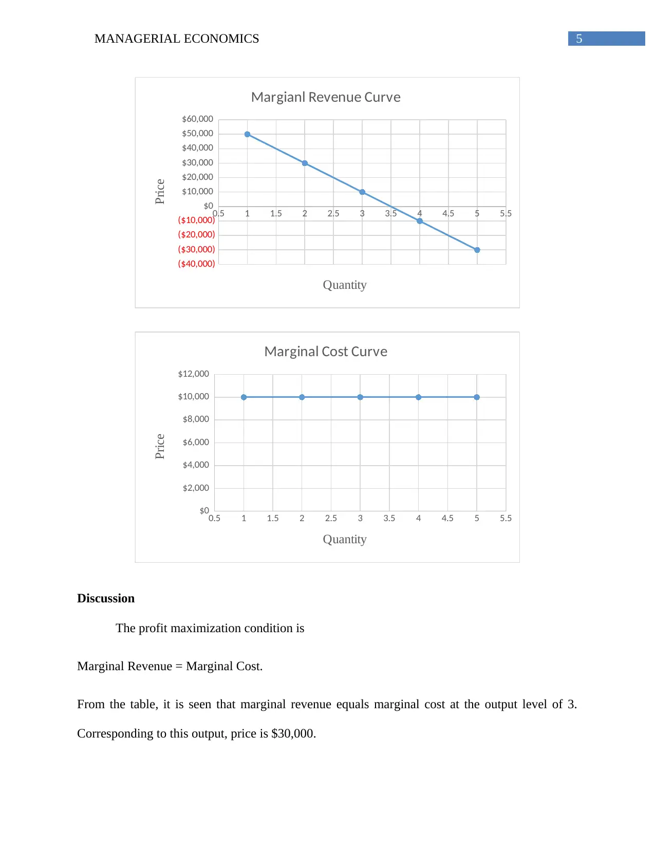
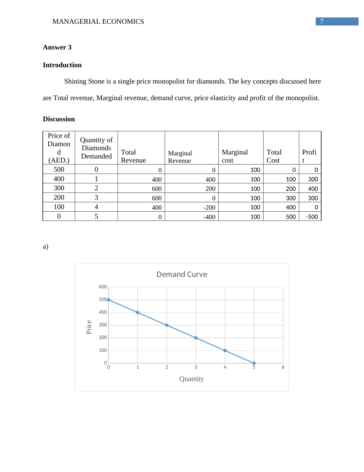
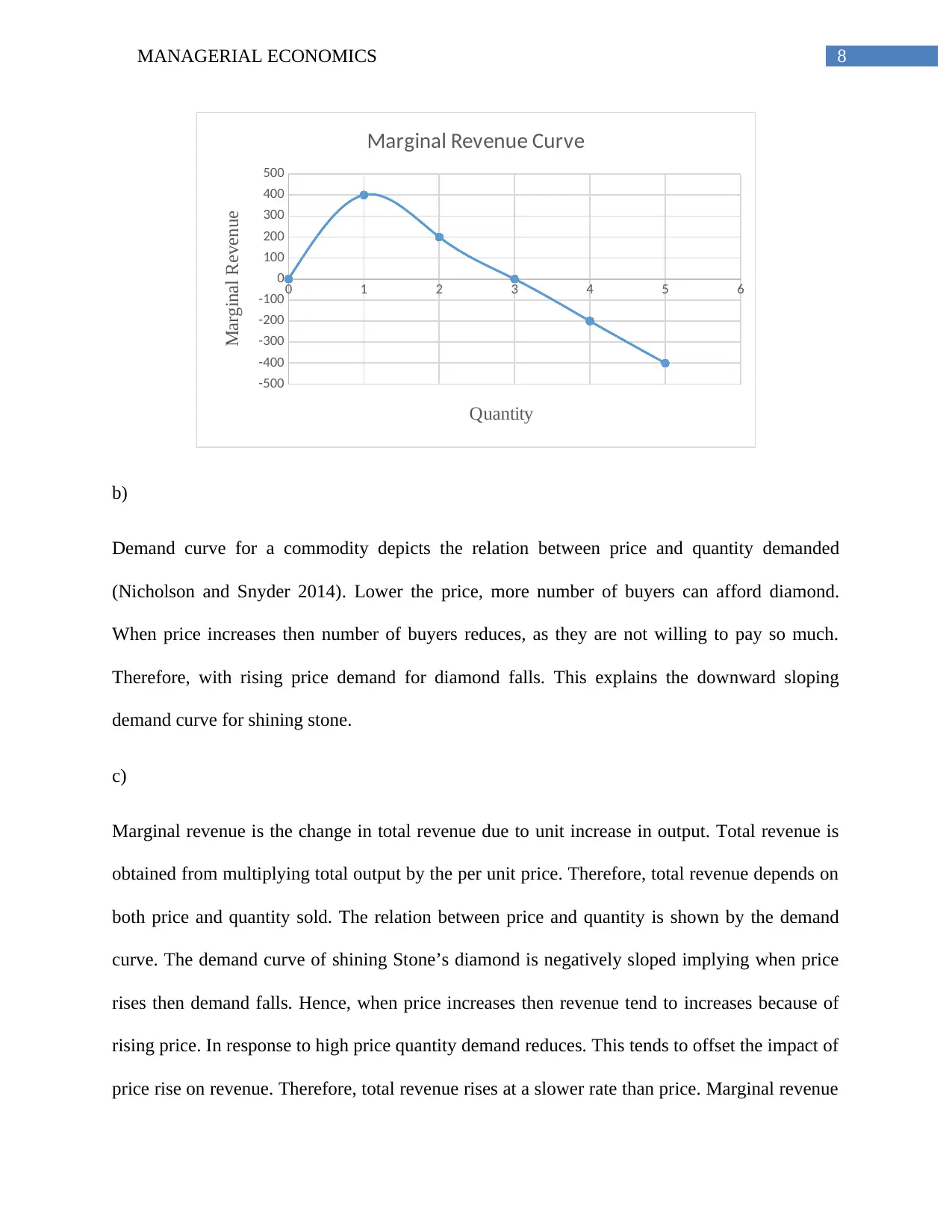
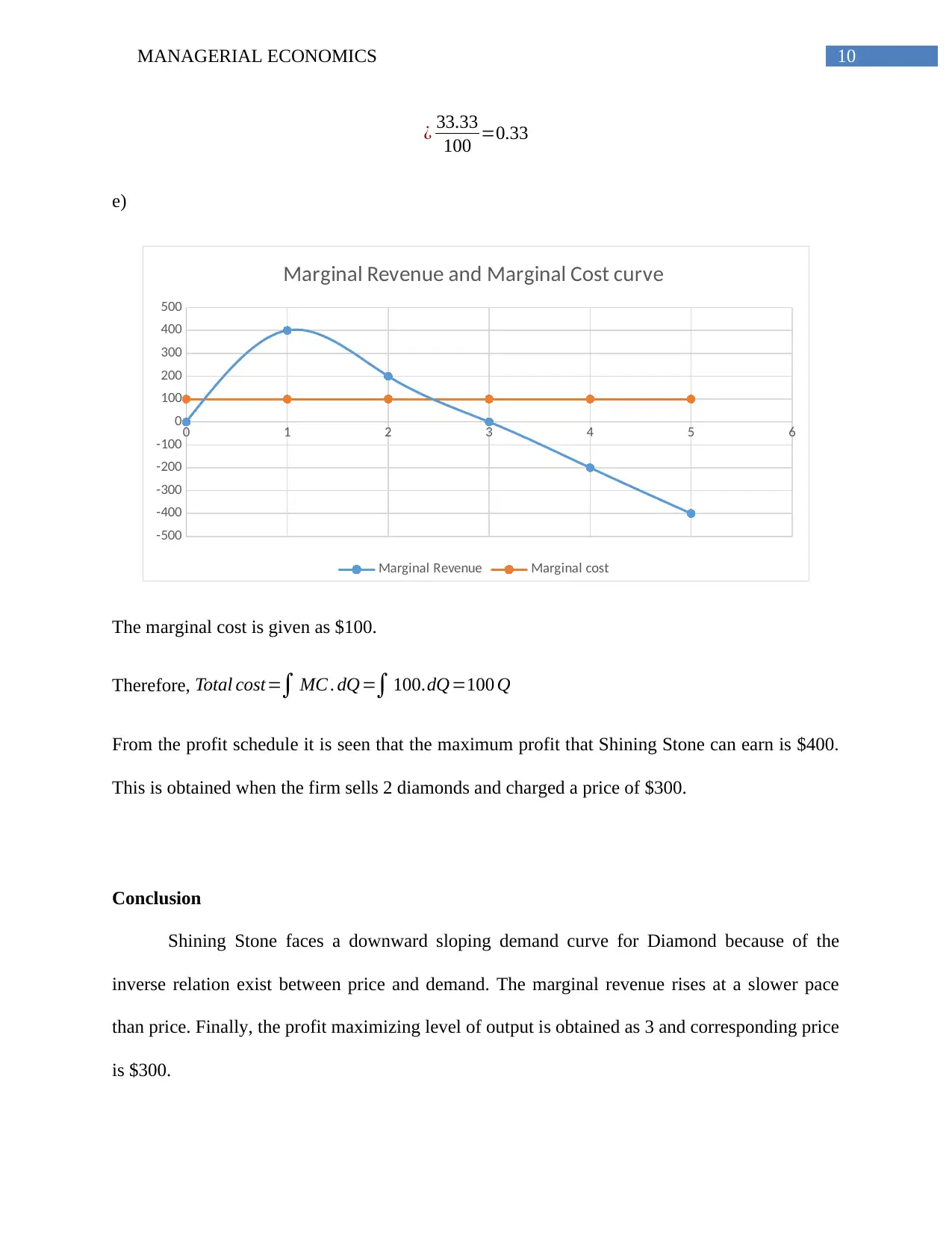
This managerial economics assignment solution analyzes the behavior of firms in different market structures, including perfect competition and monopoly. The assignment explores key concepts such as marginal cost, marginal revenue, profit maximization, and the impact of market forces on firm output and pricing decisions. The solution includes detailed calculations, graphs, and explanations to illustrate the concepts of equilibrium, excess capacity, and the relationship between price, quantity, and profit. It examines how firms make decisions in both the short run and long run, considering factors like demand, cost structures, and market competition. The assignment also discusses the concept of price elasticity and its implications for a monopolist's pricing strategy. The solution demonstrates the application of economic principles to real-world scenarios, providing a comprehensive understanding of market dynamics and firm behavior.

Running head: MANAGERIAL ECONOMICS
Managerial Economics
Name of the Student
Name of the University
Author note

1MANAGERIAL ECONOMICS
Table of Contents
Answer 1..........................................................................................................................................2
Introduction..................................................................................................................................2
Discussion....................................................................................................................................2
Conclusion...................................................................................................................................3
Answer 2..........................................................................................................................................4
Introduction......................................................................................................................................4
Graphs..........................................................................................................................................4
Discussion........................................................................................................................................5
Conclusion.......................................................................................................................................6
Answer 3..........................................................................................................................................7
Introduction..................................................................................................................................7
Discussion....................................................................................................................................7
Conclusion.................................................................................................................................10
References......................................................................................................................................11

2MANAGERIAL ECONOMICS
Answer 1
Introduction
The short run equilibrium point of a competitive firm occurs at a point where price equals
marginal cost. The profit maximizing condition reduces to the condition marginal cost condition
because price is given in the market. Competitive firm produces output which is socially optimal
and in the long run it operates at the minimum point of long run average variable cost.
Discussion
Excess capacity is a situation where firm produces output less than the optimum. It is
possible for firms if they can operate at the falling part of long run average cost. Competitive
firm in the short run produces output where price and marginal cost equalizes. In the short run, it
can enjoy supernormal profit or loss. However, because of free entry and exits, in the phase of
supernormal profit, new firms enter and reduce profit and this continues unless firms reach to the
minimum point of long run average cost. In the phase of loss firm leaves the industry and loss
recovered and exit continues until the industry achieve only normal profit (Dean 2014).
Therefore, firms in the long term always operate at the minimum point of long run average cost.
a)
Quantity Price
Total
revenu
e
Total
cost
Marginal
cost
0 $60 $0 $50 $50
1 60 $60 70 $20
2 60 $120 110 $40
3 60 $180 170 $60
4 60 $240 240 $70
5 60 $300 330 $90

3MANAGERIAL ECONOMICS
b)
Graph of MC and P
0 1 2 3 4 5 6
$0
$10
$20
$30
$40
$50
$60
$70
$80
$90
$100
Price
Marginal cost
Quantity
Price, Cost
c)
From the above demand and cost schedule the equilibrium output level is 3. The marginal cost at
this level of output is $60.
Conclusion
Perfectly competitive firm produces optimal social output. Firms retain excess capacity to
enjoy more than normal profit. Here, firms enjoy economies of scale and can operate at the
falling part of average cost. It is found only for monopolistically competitive firm. For pure
competition, firms utilizes al its capacity to produce socially optimal output.

4MANAGERIAL ECONOMICS
Answer 2
Introduction
When a firm produces the entire market supply of a particular good or service then the
firm is a monopoly firm. The monopoly makes its operation in order to maximize profit. The
Profit maximization condition requires that marginal revenue match with marginal cost. The
important term require for profit analysis are demand, marginal revenue and marginal cost.
Graphs
Price
Quantity
Demanded
Total
revenue
Marginal
Revenue
Marginal
Cost
$50,000.0
0 1 $50,000 $50,000 $10,000
$40,000.0
0 2 $80,000 $30,000 $10,000
$30,000.0
0 3 $90,000 $10,000 $10,000
$20,000.0
0 4 $80,000 ($10,000) $10,000
$10,000.0
0 5 $50,000 ($30,000) $10,000
0.5 1 1.5 2 2.5 3 3.5 4 4.5 5 5.5
$0.00
$10,000.00
$20,000.00
$30,000.00
$40,000.00
$50,000.00
$60,000.00
Demand Curve
Quantity
Price

5MANAGERIAL ECONOMICS
0.5 1 1.5 2 2.5 3 3.5 4 4.5 5 5.5
($40,000)
($30,000)
($20,000)
($10,000)
$0
$10,000
$20,000
$30,000
$40,000
$50,000
$60,000
Margianl Revenue Curve
Quantity
Price
0.5 1 1.5 2 2.5 3 3.5 4 4.5 5 5.5
$0
$2,000
$4,000
$6,000
$8,000
$10,000
$12,000
Marginal Cost Curve
Quantity
Price
Discussion
The profit maximization condition is
Marginal Revenue = Marginal Cost.
From the table, it is seen that marginal revenue equals marginal cost at the output level of 3.
Corresponding to this output, price is $30,000.

6MANAGERIAL ECONOMICS
Profit=Total Revenue−Total Cost
Given the constant marginal cost of $10,000, the total variable cost is given by
TVC =∫ 10,000.dQ
¿ 10,000 Q
Total cost function=$ 50,000+10,000 Q
At the output level of 3,
Total revenue = (3*$30,000) = $90,000
Total cost=$ 50000+ ( $ 10000∗3 )
¿ $ 50,000+$ 30,000
¿ $ 80,000
Profit=$ 90,000−$ 80,000
¿ $ 10,000
Conclusion
The profit maximizing level of output and price is 3 and $30,000 respectively. The profit
obtained by the firm is $10,000.

7MANAGERIAL ECONOMICS
Answer 3
Introduction
Shining Stone is a single price monopolist for diamonds. The key concepts discussed here
are Total revenue, Marginal revenue, demand curve, price elasticity and profit of the monopolist.
Discussion
Price of
Diamon
d
(AED.)
Quantity of
Diamonds
Demanded Total
Revenue
Marginal
Revenue
Marginal
cost
Total
Cost
Profi
t
500 0 0 0 100 0 0
400 1 400 400 100 100 300
300 2 600 200 100 200 400
200 3 600 0 100 300 300
100 4 400 -200 100 400 0
0 5 0 -400 100 500 -500
a)
0 1 2 3 4 5 6
0
100
200
300
400
500
600
Demand Curve
Quantity
Price

8MANAGERIAL ECONOMICS
0 1 2 3 4 5 6
-500
-400
-300
-200
-100
0
100
200
300
400
500
Marginal Revenue Curve
Quantity
Marginal Revenue
b)
Demand curve for a commodity depicts the relation between price and quantity demanded
(Nicholson and Snyder 2014). Lower the price, more number of buyers can afford diamond.
When price increases then number of buyers reduces, as they are not willing to pay so much.
Therefore, with rising price demand for diamond falls. This explains the downward sloping
demand curve for shining stone.
c)
Marginal revenue is the change in total revenue due to unit increase in output. Total revenue is
obtained from multiplying total output by the per unit price. Therefore, total revenue depends on
both price and quantity sold. The relation between price and quantity is shown by the demand
curve. The demand curve of shining Stone’s diamond is negatively sloped implying when price
rises then demand falls. Hence, when price increases then revenue tend to increases because of
rising price. In response to high price quantity demand reduces. This tends to offset the impact of
price rise on revenue. Therefore, total revenue rises at a slower rate than price. Marginal revenue

9MANAGERIAL ECONOMICS
which is the change in total revenue from additional sales of diamond is less than price of
diamond.
d)
At price $200, demand is 3
When price decreases from $200 to $100 then demand raises from 3 to 4 diamonds.
Therefore,
Percentage change ∈ price=Change∈ price
Initial price ∗100
¿ ( 200−100 )
100 ∗100
¿ 100
100∗100=100
There is a 100 percent change in price.
Percentage change ∈quantity= Change∈quantity demand
Initial demand ∗100
¿ ( 4−3 )
3 ∗100
¿ 1
3∗100
¿ 33.33
The percent change in quantity is 33.33%.
Price elasticity= percentage change∈demand
percentage change∈ price

10MANAGERIAL ECONOMICS
¿ 33.33
100 =0.33
e)
0 1 2 3 4 5 6
-500
-400
-300
-200
-100
0
100
200
300
400
500
Marginal Revenue and Marginal Cost curve
Marginal Revenue Marginal cost
The marginal cost is given as $100.
Therefore, Total cost=∫ MC . dQ =∫ 100.dQ =100 Q
From the profit schedule it is seen that the maximum profit that Shining Stone can earn is $400.
This is obtained when the firm sells 2 diamonds and charged a price of $300.
Conclusion
Shining Stone faces a downward sloping demand curve for Diamond because of the
inverse relation exist between price and demand. The marginal revenue rises at a slower pace
than price. Finally, the profit maximizing level of output is obtained as 3 and corresponding price
is $300.

11MANAGERIAL ECONOMICS
References
Dean, E., 2014. Principles of Microeconomics: Scarcity and Social Provisioning.
Nicholson, W. and Snyder, C.M., 2014. Intermediate microeconomics and its application.
Cengage Learning.