Managerial Economics Assignment: Regression, Elasticity & Profit

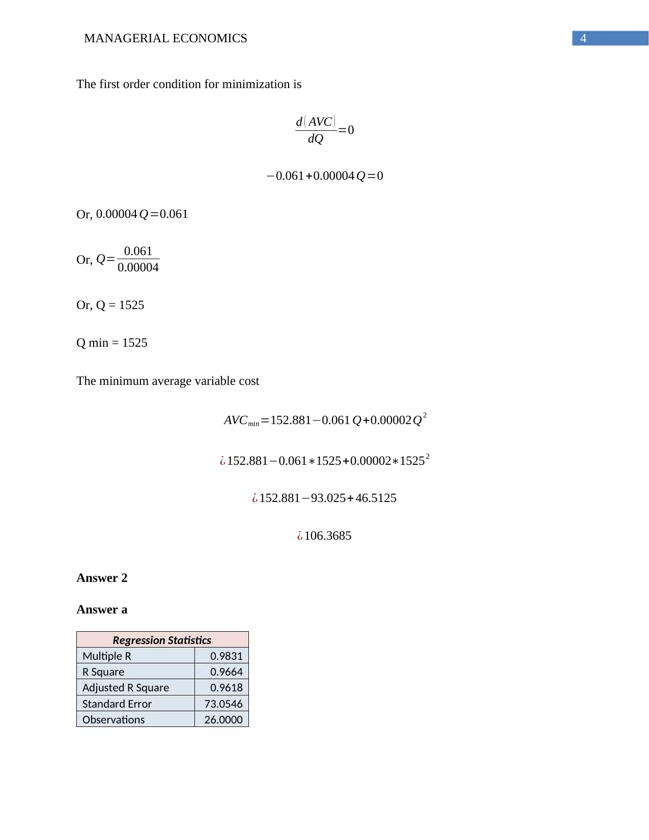
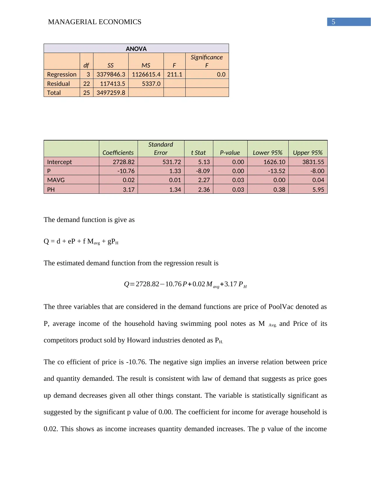
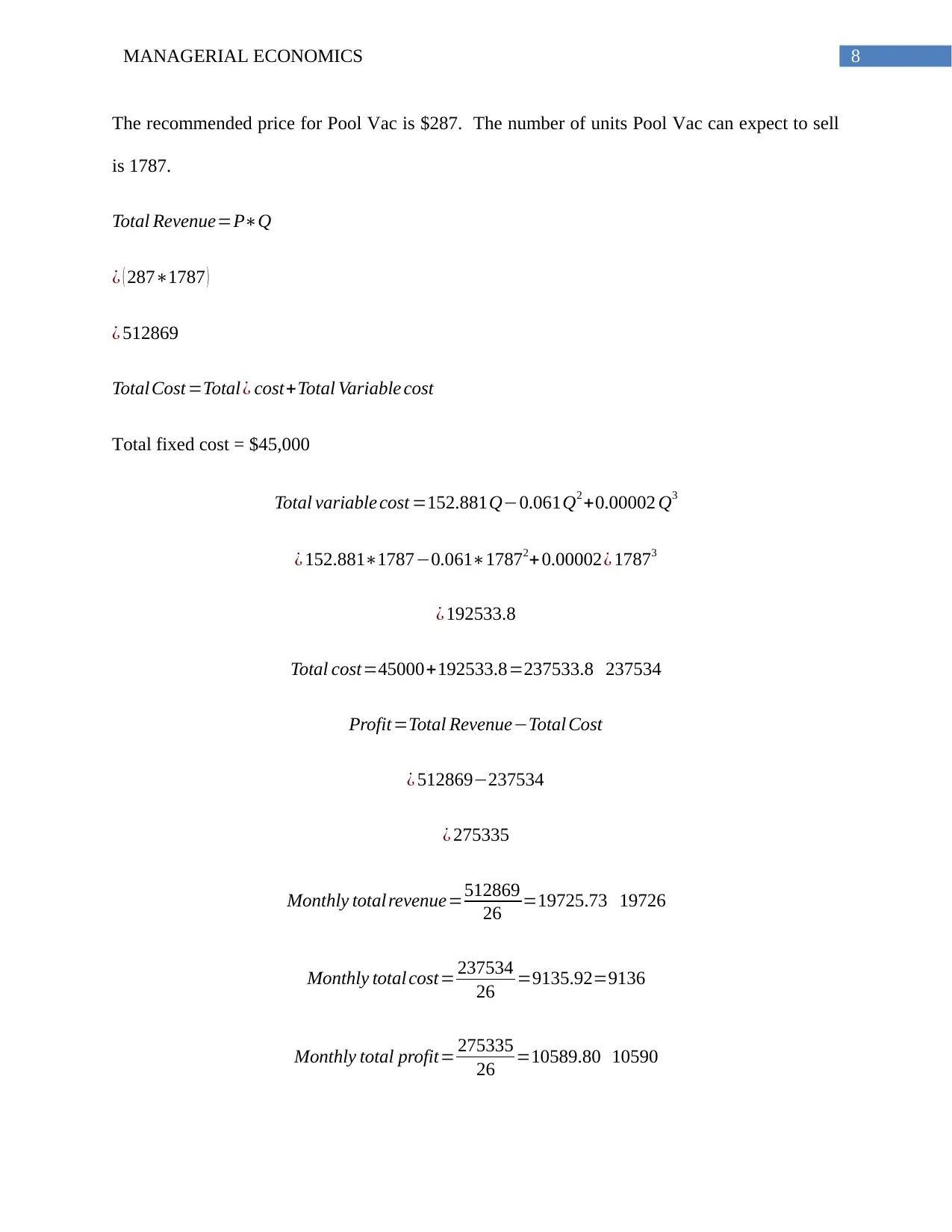
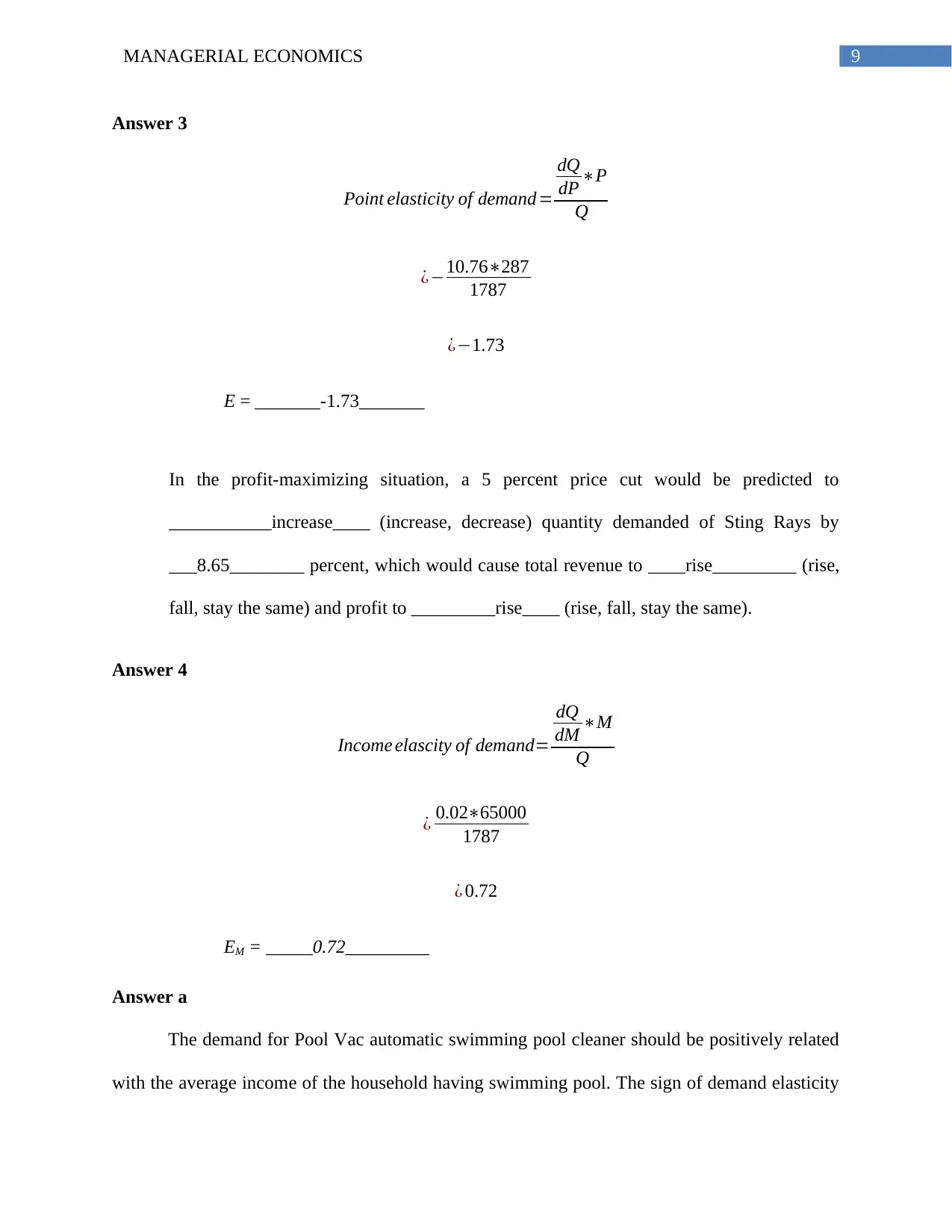
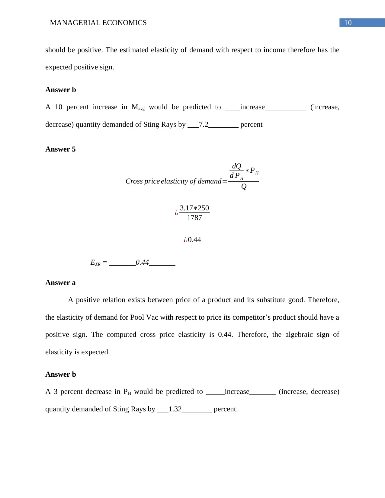
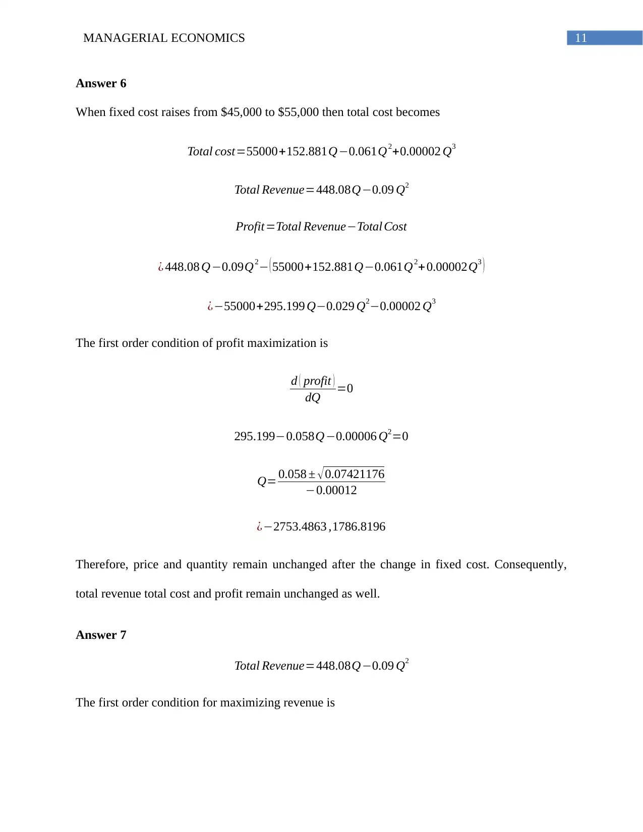
This document provides a comprehensive solution to a managerial economics assignment. The solution includes regression analysis to determine the relationship between average variable cost and quantity, deriving the average variable cost, total variable cost, and marginal cost functions. It also analyzes a demand function, considering factors like price, average household income, and competitor's prices, and calculates the optimal price and quantity for profit maximization. Furthermore, the assignment explores elasticity concepts, including price, income, and cross-price elasticities, and assesses the impact of price changes on demand and revenue. The document also examines the effects of changes in fixed costs and provides insights into revenue maximization strategies.

Running head: MANAGERIAL ECONOMICS
Managerial Economics
Name of the Student
Name of the University
Author note

1MANAGERIAL ECONOMICS
Table of Contents
Answer 1..........................................................................................................................................2
Answer a......................................................................................................................................2
Answer b......................................................................................................................................3
Answer c......................................................................................................................................3
Answer 2..........................................................................................................................................4
Answer a......................................................................................................................................4
Answer b......................................................................................................................................6
Answer c......................................................................................................................................7
Answer 3..........................................................................................................................................8
Answer 4..........................................................................................................................................9
Answer a......................................................................................................................................9
Answer b....................................................................................................................................10
Answer 5........................................................................................................................................10
Answer a....................................................................................................................................10
Answer b....................................................................................................................................10
Answer 6........................................................................................................................................10
Answer 7........................................................................................................................................11

2MANAGERIAL ECONOMICS
Answer 1
Answer a
Regression Statistics
Multiple R
0.8
0
R Square
0.6
3
Adjusted R Square
0.6
0
Standard Error
7.7
3
Observations 26
ANOVA
df SS MS F
Significance
F
Regression 2 2387.498 1193.749 19.975 0.000
Residual 23 1374.541 59.763
Total 25 3762.038
Coefficient
s
Standard
Error t Stat
P-
value Lower 95%
Upper
95%
Intercept 152.881 6.605 23.146 0.000 139.217 166.544
Q -0.061 0.015 -4.199 0.000 -0.092 -0.031
Q2 0.00002 0.000 2.693 0.013 0.000 0.000
The regression result shows the estimated relation between average variable cost and quantity.
The value of intercept a = 152.881. The p value is 0.0000. This means the intercept is statistically
significant. The coefficient of Q is b = -0.061. This implies with a rise in quantity average
variable cost decreases. This is what happens at the early stages of production. The P value for
the variable is 0.000 implying statistical significance of quantity. The next variable in the
Average cost function is Q2. The estimated coefficient is c= 0.00002. The positive sign of the

3MANAGERIAL ECONOMICS
parameter shows a positive relation between average variable cost and Q2. The implication is that
as quantity starts increasing at a rapid rate then cost also increases. The P value is 0.013. As the p
value is less than 0.05, the variable Q2 is statistically significant.
Answer b
The Average Variable Cost function is
AVC=152.881−0.061Q+0.00002 Q2
The Total Variable Cost Function is Quantity times the average variable cost.
TVC = Q*AVC
= Q (a + b Q + cQ2)
TVC =Q(152.881−0.061 Q+0.00002Q2 )
¿ 152.881Q−0.061 Q2+0.00002Q3
The Marginal Cost Function is the change in total cost due to unit change in quantity. The
marginal cost function is obtained as
MC= d (TVC )
dQ
¿ d (152.881Q−0.061Q2 +0.00002 Q3)
dQ
¿ 152.881−0.122 Q+0.00006 Q2
Answer c
AVC = 152.881 – 0.061Q + 0.00002Q2

4MANAGERIAL ECONOMICS
The first order condition for minimization is
d ( AVC )
dQ =0
−0.061+0.00004 Q=0
Or, 0.00004 Q=0.061
Or, Q= 0.061
0.00004
Or, Q = 1525
Q min = 1525
The minimum average variable cost
AVCmin=152.881−0.061 Q+0.00002Q2
¿ 152.881−0.061∗1525+0.00002∗15252
¿ 152.881−93.025+ 46.5125
¿ 106.3685
Answer 2
Answer a
Regression Statistics
Multiple R 0.9831
R Square 0.9664
Adjusted R Square 0.9618
Standard Error 73.0546
Observations 26.0000

5MANAGERIAL ECONOMICS
ANOVA
df SS MS F
Significance
F
Regression 3 3379846.3 1126615.4 211.1 0.0
Residual 22 117413.5 5337.0
Total 25 3497259.8
Coefficients
Standard
Error t Stat P-value Lower 95% Upper 95%
Intercept 2728.82 531.72 5.13 0.00 1626.10 3831.55
P -10.76 1.33 -8.09 0.00 -13.52 -8.00
MAVG 0.02 0.01 2.27 0.03 0.00 0.04
PH 3.17 1.34 2.36 0.03 0.38 5.95
The demand function is give as
Q = d + eP + f Mavg + gPH
The estimated demand function from the regression result is
Q=2728.82−10.76 P+ 0.02 M avg +3.17 PH
The three variables that are considered in the demand functions are price of PoolVac denoted as
P, average income of the household having swimming pool notes as M Avg. and Price of its
competitors product sold by Howard industries denoted as PH.
The co efficient of price is -10.76. The negative sign implies an inverse relation between price
and quantity demanded. The result is consistent with law of demand that suggests as price goes
up demand decreases given all other things constant. The variable is statistically significant as
suggested by the significant p value of 0.00. The coefficient for income for average household is
0.02. This shows as income increases quantity demanded increases. The p value of the income

6MANAGERIAL ECONOMICS
variable is 0.03. As the value less than 0.05, therefore the variable is statistically significant at
5% level of significance. The co efficient of the price of the competitor pool cleaner product
Howard industries is 3.17. In case of substitute goods, increase in the price of one goods raises
the demand for its substitute product. This explains the rationale for having positive relation
between Pool Vac’s demand and price of competitive pool cleaner product. The significant p
value of 0.03 of PH means the Pool Vac’s demand has a positive significant relation with price of
Howard industries cleaner product.
Answer b
If Howard industry charges a price of $250, and expected average, household income is $65,000,
and then the estimated demand function is
Q=2728.82−10.76 P+ 0.02 M avg +3.17 PH
¿ 2728.82−10.76 P+0.02∗65000+3.17∗250
¿ 2728.82−10.76 P+1300+792.5
¿ 4821.32−10.76 P
Inverse demand function is given as
P= 4821.32−Q
10.76
¿ 448.08−0.09 Q
Total revenue
TR=P∗Q
¿ ( 448.08−0.09 Q )∗Q

7MANAGERIAL ECONOMICS
¿ 448.08 Q−0.09Q2
Marginal Revenue
MR= dTR
dQ
¿ d (448.08 Q−0.09Q2 )
dQ
¿ 448.08−0.18 Q
Answer c
The profit maximization condition of the firm is,
MR = MC
448.08−0.18 Q=152.881−0.122Q+0.00006 Q2
Or, −0.00006 Q2−0.058 Q+295.199=0
Q= 0.058 ± √0.07421176
−0.00012
¿−2753.4863 ,1786.8196
Q = 1786.8196 ~ 1787
P = 448.08−0.09 Q
¿ 448.08− ( 0.09∗1787 )
¿ 287.25 287

8MANAGERIAL ECONOMICS
The recommended price for Pool Vac is $287. The number of units Pool Vac can expect to sell
is 1787.
Total Revenue=P∗Q
¿ ( 287∗1787 )
¿ 512869
Total Cost =Total ¿ cost+Total Variable cost
Total fixed cost = $45,000
Total variable cost =152.881Q−0.061Q2 +0.00002 Q3
¿ 152.881∗1787−0.061∗17872+ 0.00002¿ 17873
¿ 192533.8
Total cost=45000+192533.8=237533.8 237534
Profit=Total Revenue−Total Cost
¿ 512869−237534
¿ 275335
Monthly total revenue=512869
26 =19725.73 19726
Monthly total cost= 237534
26 =9135.92=9136
Monthly total profit= 275335
26 =10589.80 10590

9MANAGERIAL ECONOMICS
Answer 3
Point elasticity of demand=
dQ
dP ∗P
Q
¿−10.76∗287
1787
¿−1.73
E = _______-1.73_______
In the profit-maximizing situation, a 5 percent price cut would be predicted to
___________increase____ (increase, decrease) quantity demanded of Sting Rays by
___8.65________ percent, which would cause total revenue to ____rise_________ (rise,
fall, stay the same) and profit to _________rise____ (rise, fall, stay the same).
Answer 4
Income elascity of demand=
dQ
dM ∗M
Q
¿ 0.02∗65000
1787
¿ 0.72
EM = _____0.72_________
Answer a
The demand for Pool Vac automatic swimming pool cleaner should be positively related
with the average income of the household having swimming pool. The sign of demand elasticity

10MANAGERIAL ECONOMICS
should be positive. The estimated elasticity of demand with respect to income therefore has the
expected positive sign.
Answer b
A 10 percent increase in Mavg would be predicted to ____increase___________ (increase,
decrease) quantity demanded of Sting Rays by ___7.2________ percent
Answer 5
Cross price elasticity of demand=
dQ
d PH
∗PH
Q
¿ 3.17∗250
1787
¿ 0.44
EXR = _______0.44_______
Answer a
A positive relation exists between price of a product and its substitute good. Therefore,
the elasticity of demand for Pool Vac with respect to price its competitor’s product should have a
positive sign. The computed cross price elasticity is 0.44. Therefore, the algebraic sign of
elasticity is expected.
Answer b
A 3 percent decrease in PH would be predicted to _____increase_______ (increase, decrease)
quantity demanded of Sting Rays by ___1.32________ percent.

11MANAGERIAL ECONOMICS
Answer 6
When fixed cost raises from $45,000 to $55,000 then total cost becomes
Total cost=55000+152.881Q−0.061Q2+0.00002 Q3
Total Revenue=448.08Q−0.09 Q2
Profit=Total Revenue−Total Cost
¿ 448.08 Q−0.09Q2− ( 55000+152.881Q−0.061Q2+0.00002Q3 )
¿−55000+295.199 Q−0.029 Q2−0.00002 Q3
The first order condition of profit maximization is
d ( profit )
dQ =0
295.199−0.058Q−0.00006 Q2=0
Q= 0.058 ± √0.07421176
−0.00012
¿−2753.4863 ,1786.8196
Therefore, price and quantity remain unchanged after the change in fixed cost. Consequently,
total revenue total cost and profit remain unchanged as well.
Answer 7
Total Revenue=448.08Q−0.09 Q2
The first order condition for maximizing revenue is