Macquarie University MGNT603: Managing Finance - Pricing Analysis

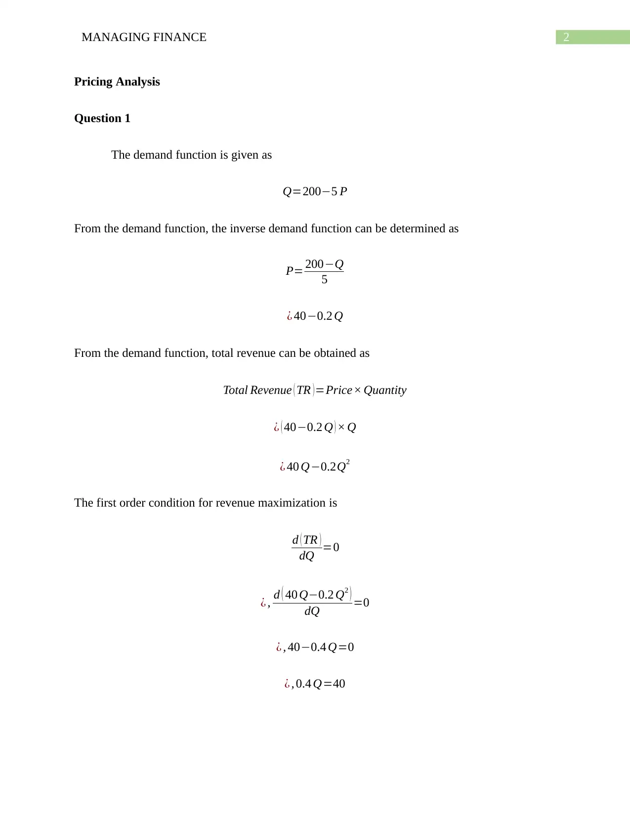
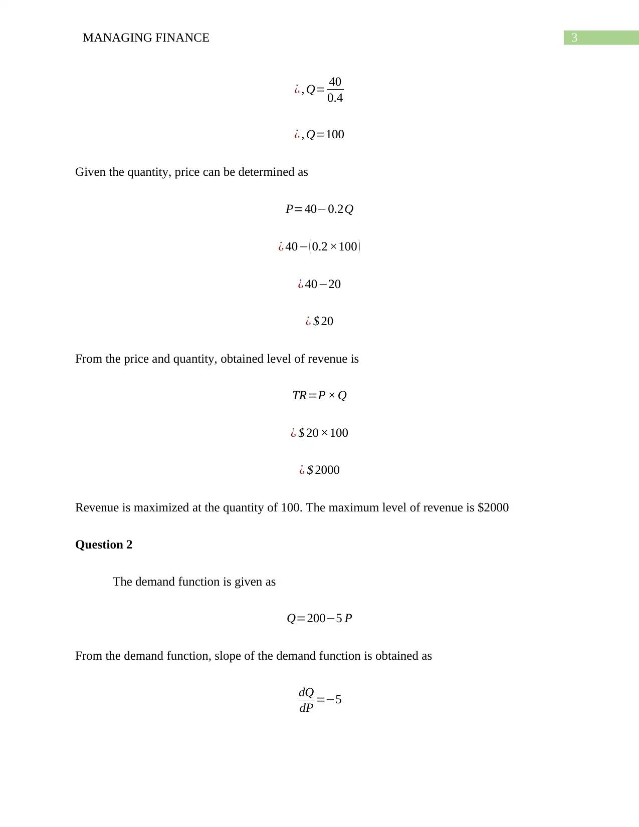
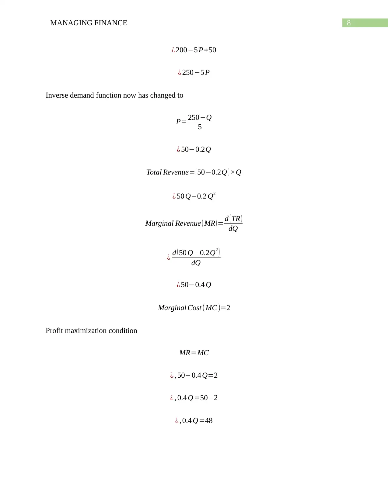
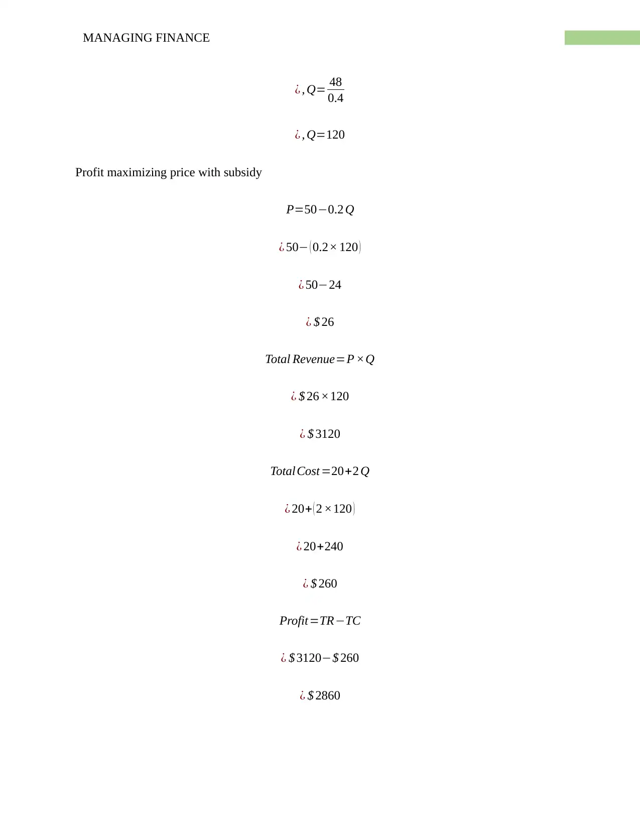
This report presents a detailed pricing analysis for an automotive manufacturing company, Bolden, addressing key financial concepts within a scenario-based case study. It begins by deriving the inverse demand function from a given demand function and determining the quantity at which revenue is maximized, calculating the maximum revenue achievable. The report then examines the price elasticity of demand, analyzing the impact of price changes on total revenue and determining whether the company should lower its price based on the elasticity. The analysis extends to profit maximization, calculating the equilibrium quantity and price, and evaluating the impact of a government subsidy on the company's profit-maximizing output, price, and overall profitability. Finally, the report assesses the implications of removing the subsidy and discusses the broader economic effects of subsidies, including their impact on resource allocation and potential deadweight loss. The report provides a comprehensive understanding of pricing strategies, demand dynamics, and the financial implications of government interventions.

Running head: MANAGING FINANCE
Managing Finance
Name of the Student
Name of the University
Course ID

1MANAGING FINANCE
Table of Contents
Pricing Analysis...............................................................................................................................2
Question 1....................................................................................................................................2
Question 2....................................................................................................................................3
Question 3....................................................................................................................................4
Question 4....................................................................................................................................4
Question 5....................................................................................................................................5
Question 6....................................................................................................................................7
Question 7..................................................................................................................................10
Question 8..................................................................................................................................10

2MANAGING FINANCE
Pricing Analysis
Question 1
The demand function is given as
Q=200−5 P
From the demand function, the inverse demand function can be determined as
P= 200−Q
5
¿ 40−0.2 Q
From the demand function, total revenue can be obtained as
Total Revenue ( TR )=Price× Quantity
¿ ( 40−0.2 Q ) × Q
¿ 40 Q−0.2Q2
The first order condition for revenue maximization is
d ( TR )
dQ =0
¿ , d ( 40 Q−0.2 Q2 )
dQ =0
¿ , 40−0.4 Q=0
¿ , 0.4 Q=40

3MANAGING FINANCE
¿ , Q= 40
0.4
¿ , Q=100
Given the quantity, price can be determined as
P=40−0.2Q
¿ 40− ( 0.2 ×100 )
¿ 40−20
¿ $ 20
From the price and quantity, obtained level of revenue is
TR=P × Q
¿ $ 20 ×100
¿ $ 2000
Revenue is maximized at the quantity of 100. The maximum level of revenue is $2000
Question 2
The demand function is given as
Q=200−5 P
From the demand function, slope of the demand function is obtained as
dQ
dP =−5

4MANAGING FINANCE
Price elasticity of demand= dQ
dP × P
Q
¿−5 × 20
100
¿−1
Question 3
At price $15, quantity demanded is obtained as
Q=200−5 P
¿ 200− ( 5× 15 )
¿ 200−75
¿ 125
At this price, the computed price elasticity of demand is
Price elasticity of demand= dQ
dP × P
Q
¿−5 × 15
125
¿−5 ×0.12
¿ 0.6
Question 4
At price of $15, total revenue of the firm is
Total Revenue=$ 15 ×125

5MANAGING FINANCE
¿ $ 1875
The price of $15 is lower than profit maximizing price of $20. With a fall in price, quantity
demanded of the firm increases to 125. Price elasticity of demand at this price is 0.6. As the
measured elasticity is less than 1, it indicates a relatively inelastic demand. This mean
proportionate change in quantity demanded at this price is less than proportionate change in
price. Therefore, an increase in quantity demanded of the good following the decline in price is
proportionally less than decline in price. Because of this, decline in revenue due to a lower price
cannot be compensated by an increase in quantity demanded. The overall impact of price
decrease is therefore a decline in revenue of the firm. Under condition of price inelastic demand,
firm should not lower price. From the given scenario, it is obtained that revenue of the firm is
maximized at a price of $20 and corresponding quantity is 100. At this price and quantity, firm
earns a maximum revenue of $2000. However, if price lowers to $15, quantity demanded
increases to 125. Revenue of the form lowers to $1875. The revenue declines at price $15, the
firm can produce at this price as price is greater than variable cost.
Question 5
Total Revenue of the company is obtained as
TR=P × Q
¿ ( 40−0.2 Q ) × Q
¿ 40 Q−0.2Q2
From the total revenue function marginal revenue can be derived as
MR= d ( TR )
dQ

6MANAGING FINANCE
¿ d ( 40 Q−0.2 Q2 )
dQ
¿ 40−0.4 Q
Total cost of the organization is given as
TC=20+2 Q
Marginal cost of the company is
MC= d ( TC )
dQ
¿ d ( 20+ 2Q )
dQ
¿ 2
Profit maximization condition of the company is given as
MR=MC
¿ , 40−0.4 Q=2
¿ , 0.4 Q=38
¿ , Q=95
Equilibrium quantity that maximizes profit of the company is 95.
Corresponding to the equilibrium quantity, equilibrium price is obtained as
P=40−0.2Q
¿ 40− ( 0.2 ×95 )

7MANAGING FINANCE
¿ 40−19
¿ $ 21
At equilibrium, market price is $21 and equilibrium quantity is 95.
Total Revennue=$ 21× 95
¿ $ 1995
Total cost to produce equilibrium quantity of output is
Total Cost =20+2 Q
¿ 20+ ( 2 ×95 )
¿ 20+190
¿ $ 210
Obtained profit corresponding to equilibrium price and quantity is
Profit=Total Revenue−Total Cost
¿ $ 1995−$ 21 0
¿ $ 1785
Question 6
If government provides a subsidy of $10 for every unit sold, then vehicles are available at
the market a lower price. Price reduces by $10 for every unit sold. The new demand function
then is obtained as
Q=200−5 ( P−10 )

8MANAGING FINANCE
¿ 200−5 P+50
¿ 250−5 P
Inverse demand function now has changed to
P= 250−Q
5
¿ 50−0.2Q
Total Revenue= ( 50−0.2Q ) ×Q
¿ 50 Q−0.2 Q2
Marginal Revenue ( MR ) = d ( TR )
dQ
¿ d (50 Q−0.2Q2 )
dQ
¿ 50−0.4 Q
Marginal Cost (MC )=2
Profit maximization condition
MR=MC
¿ , 50−0.4 Q=2
¿ , 0.4 Q=50−2
¿ , 0.4 Q=48

9MANAGING FINANCE
¿ , Q= 48
0.4
¿ , Q=120
Profit maximizing price with subsidy
P=50−0.2 Q
¿ 50− ( 0.2× 120 )
¿ 50−24
¿ $ 26
Total Revenue=P ×Q
¿ $ 26 ×120
¿ $ 3120
Total Cost =20+2 Q
¿ 20+ ( 2 ×120 )
¿ 20+240
¿ $ 260
Profit=TR−TC
¿ $ 3120−$ 260
¿ $ 2860

10MANAGING FINANCE
The subsidy increases profit maximizing output to 120. Price that sellers receive increases to $26
resulting in a higher profit of $2860 for the company.
Question 7
If the government stopped the subsidy, then the company has to sell vehicles at a lower
price of $21 and earn a relatively lower profit of $1785 rather than a much higher profit with
subsidy.
Question 8
Subsidy is not a good thing for the overall market as it results in a socially inefficient
allocation of resources. Firstly, the subsidy imposes a huge cost to the government. Given a $10
subsidy to every unit sell, total cost of subsidy to the government is ($10 * 120) = $1200.
Secondly, subsidy results in a deadweight or welfare loss due to economic inefficiency. Subsidy
distorts the allocation of resources. The resulted deadweight loss is 2*0.5*5*(120 – 95) = 125.
Subsidy is a bad thing for the overall market as because of subsidy too much resources of the
society is devoted for fewer amount of goods.

11MANAGING FINANCE