MAR8067 Marine Machinery Systems: Analyzing and Stabilizing Systems

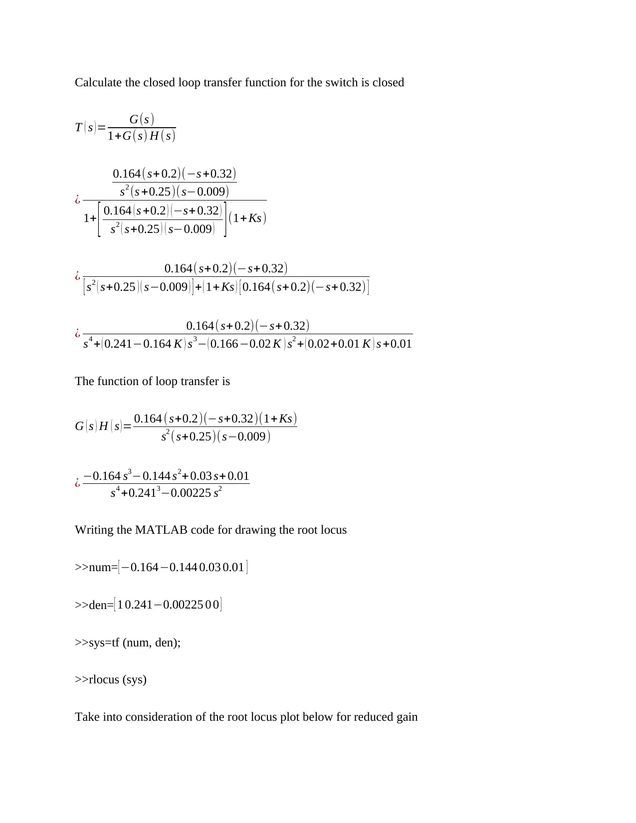
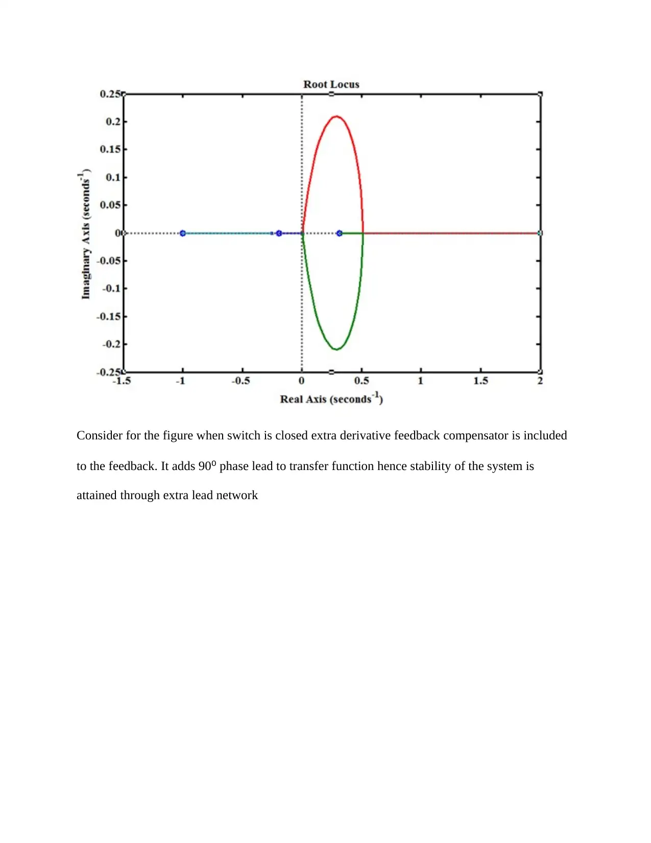
This report provides a detailed analysis of marine machinery systems, focusing on closed-loop systems and stability analysis. It begins with determining the closed-loop block diagram and transfer function for a hydraulic servomechanism with mechanical feedback. The report then analyzes the stability of a given system using Bode plots, pole-zero maps, and root locus techniques, concluding that the system is unstable. Furthermore, it explores methods to stabilize the system, including the use of proportional feedback compensators, and discusses the design and implementation of appropriate feedback controllers. The report includes MATLAB code snippets and relevant plots to support the analysis and findings. Desklib offers a wealth of similar solved assignments for students.

MAR8067 MARINE MACHINERY SYSTEMS
By Name
Course
Instructor
Institution
Location
Date

Question 1
(a) closed-loop block diagram for this mechanical system
In problem statement it is provided that from geometry
∆ z=k l1−l2
l1
( x− y ) −l2
l1
y … … … … … … ..(1)
The flow rate balance gives
A dy
dt p . ∆ z
Applying Laplace transform

AsY ( s ) = p ∆ z (s )
Y ( s )= ∆ z ( s)
As
Substituting equation 1in the equation above
Y ( s ) = p
As [ l1−l2
l1 ( X ( s ) −Y ( s ) ¿−l2
l1
Y (s) ) ]
Input to system is X(s)
Output to system is Y(s)
The signal flow graph of the system is as shown
(b) closed-loop transfer function
The transfer function Y (s)
X ( s) may be obtained using the Mason’s gain formula
Gain= ∑
i
Pi ∆i
∆
in which
P is the forward path gain
I is the number of forwards paths

Loops in the signal flow graph is
L1= p l2
A sl1
L2= k (l1−l2 )
l1 As
The value of ∆ in Mason’s Gain formula (to get the transfer function) is provided by
∆=1−(l1+ l2)
∆=1+ p l2
A sl1
+ k (l1−l2)
l1 As p
Forward paths from X(s) to Y(s)
p1= k (l1−l2 )
l1 As p
∆1=1 For P1
The transfer function is T = Pi ∆i
∆
X (s)
Y ( s) =
k (l1−l2 )
l1 As p
1+ p l2
A sl1
+ k (l1−l2 )
l1 As p
X (s)
Y ( s) = k (l1−l2 ) p
l1 As+ p l2 +k (l1 −l2) p

X (s)
Y ( s) =
k (l1 −l2)
l1 A p
s+ p l2
A l1
+ k (l1−l2 ) p
A l1
Hence the transfer function of the provided system is
X (s)
Y ( s) =
k (l1 −l2)
l1 A p
s+ p l2
A l1
+ k (l1−l2 ) p
A l1
Question 2
(a) Bode diagram of this system
With reference the figure for block diagram
Write the open loop transfer function of the system
G ( s )=−0.164 (s +0.2)(s−0.32)
s2 (s+0.25)( s−0.009)
¿ 0.164(s+ 0.2)(−s+ 0.32)
s2 (s +0.25)(s−0.009)
Calculate the closed loop transfer function for switch is opened
T ( s )= G(s)
1+G(s)

0.164(s+ 0.2)(−s+ 0.32)
s2 (s +0.25)(s−0.009)
1+ 0.164 (s+0.2)(−s+0.32)
s2 (s+ 0.25)( s−0.009)
¿ 0.164 ( s+0.2)(−s+0.32)
s2 ( s+0.25 ) ( s−0.009 ) +0.164 (s +0.2)(−s +0.32)
The MATLAB code for drawing the pole zero plot for stability of the system
>>num= [ −0.164 0.02 0.01 ]
>>den= [ 1 0.241−0.166 0.20 0.01 ]
>>sys=tf (num, den);
>>pzmap (sys)
Consider the pole-zero plot
(b) Is this system stable?

Observe from the pole-zero maps that some poles of the closed loop transfer function is on the
right half of the s-plane
Hence the system is unstable
(b) The function of the open loop transfer is
G ( s )= −0.164 s2 +0.02 s2 +0.01
s4 +0.2341 s3−0.00225 s2
Writing the MATLAB code to draw root locus
>>number= [ −0.164 0.02 0.01 ]
>>den= [ 1 0.241−0.00225 0 0 ]
>>sys=tf (num, den);

>>rlocus (sys)
(c) Is it possible to stabilize this system by changing the gain of the transfer function G(s)?
Consider the root locus plot below for reduced gain
Observe from the root locus the loop gain is lowered, the overshoot as well reduce stating the
system did not gain stability
The system hence cannot get stabilized
(c) To attain stability of the system, proportional feedback compensator should be given
The function of the closed loop transfer is
L ( s ) = T (s )
1+ KT ( s)

¿
−0.164 s2 +0.02 s+ 0.01
s4 + 0.214 s3−0.166 s2 +0.02 s +0.01
1+ K −0.164 s2+ 0.02 s+ 0.01
s4 + 0.214 s3−0.166 s2 +0.02 s +0.01
¿ −0.164 s2+0.02 s+0.01
s4 +0.214 s3 −0.166 s2 +0.02 s+ 0.01+ K (−0.164 s2 +0.02 s+0.01)
¿ −0.164 s2 +0.02 s+ 0.01
s4 +0.214 s3 − ( 0.166+0.164 K ) s2 +0.02 ( 1+ K ) s+0.01(1+ K )
The characteristic equation is
s4 +0.214 s3− ( 0.166+ 0.164 K ) s2+ 0.02 ( 1+ K ) s+0.01 ( 1+K )=0
Through adjusting the value of K to the roots lies on negative real axis
The system gets stabilized through using proportional feedback controller even though not
derivative controller
Hence, it is not possible to stabilize the system with derivative controller
(d) The suitable feedback controller is proportional feedback controller
Hence the system is stabilized using proportional feedback compensator
(e) Write open loop transfer function of system
G ( s )= 0.164( s+ 0.2)(−s +0.32)
s2 (s +0.25)( s−0.009)
Calculating the feedback transfer function for the switch is closed
H(s) =1+Ks

Calculate the closed loop transfer function for the switch is closed
T ( s )= G(s )
1+G(s) H ( s)
¿
0.164( s+ 0.2)(−s +0.32)
s2 (s +0.25)( s−0.009)
1+ [ 0.164 ( s +0.2 ) (−s+ 0.32 )
s2 ( s+0.25 ) ( s−0.009 ) ](1+Ks)
¿ 0.164( s+0.2)(−s+0.32)
[ s2 ( s+0.25 ) ( s−0.009 ) ] + ( 1+ Ks ) [ 0.164(s+ 0.2)(−s+0.32) ]
¿ 0.164( s+ 0.2)(−s+ 0.32)
s4 + ( 0.241−0.164 K ) s3− ( 0.166−0.02 K ) s2 + ( 0.02+0.01 K ) s +0.01
The function of loop transfer is
G ( s ) H ( s ) = 0.164 ( s+0.2)(−s+0.32)(1+ Ks)
s2 ( s+0.25)(s−0.009)
¿ −0.164 s3−0.144 s2+ 0.03 s+ 0.01
s4 +0.2413−0.00225 s2
Writing the MATLAB code for drawing the root locus
>>num= [−0.164−0.144 0.03 0.01 ]
>>den= [ 1 0.241−0.00225 0 0 ]
>>sys=tf (num, den);
>>rlocus (sys)
Take into consideration of the root locus plot below for reduced gain

Consider for the figure when switch is closed extra derivative feedback compensator is included
to the feedback. It adds 90⁰ phase lead to transfer function hence stability of the system is
attained through extra lead network

References
Emovon, I., Norman, R.A. and Murphy, A.J., 2016. An integration of multi-criteria decision
making techniques with a delay time model for determination of inspection intervals for marine
machinery systems. Applied Ocean Research, 59, pp.65-82
Georgopoulou, C.A., Dimopoulos, G.G. and Kakalis, N.M., 2016. Modelling and simulation of a
marine propulsion power plant with seawater desulphurisation scrubber. Proceedings of the
Institution of Mechanical Engineers, Part M: Journal of Engineering for the Maritime
Environment, 230(2), pp.341-353