Marketing Research Report: SPSS Analysis & Customer Loyalty Factors
VerifiedAdded on 2023/01/11
|13
|3071
|100
Report
AI Summary
This report presents a comprehensive marketing research analysis conducted using SPSS. It investigates several key areas, including the impact of employment status on fitness hours, the association between income and gambling expenditure, the relationship between age and attitudes toward university qualifications, and preferences for cycling versus running articles. The analysis employs various statistical tests such as independent samples t-tests, correlation tests, homogeneity of variances, paired t-tests, and Chi-square tests to derive meaningful insights. Furthermore, the report explores the variables influencing customer loyalty through regression analysis, identifying satisfaction, friendliness of staff, and gift card offers as significant factors. The report provides detailed results, interpretations, and conclusions for each research question, offering valuable insights for marketing professionals and researchers. The analysis aims to provide insights for a regional health advisory association, a national budgeting service organization, a tertiary education advisory board, and a new magazine, Cycling n’ Running NZ.

Marketing Research (SPSS)
1
1
Paraphrase This Document
Need a fresh take? Get an instant paraphrase of this document with our AI Paraphraser
Contents
QUESTION 1..................................................................................................................................1
Determining if any differences exist in the number of hours spent working out last year
between employed and unemployed people................................................................................1
QUESTION 2..................................................................................................................................2
Identifying that whether there an association between total personal income and their spend on
gambling......................................................................................................................................2
QUESTION 3..................................................................................................................................3
Determining the relationship between age and attitude toward gaining a university
qualification.................................................................................................................................3
QUESTION 4..................................................................................................................................4
Identifying whether there is a difference in the extent of preference for articles about cycling
compared to articles about running..............................................................................................4
QUESTION 5..................................................................................................................................8
(a) Variables that demonstrate a significant relationship with customer loyalty.........................8
(b) Regression model...................................................................................................................9
(c) Predicting customer loyalty..................................................................................................10
(d) Overall model fit..................................................................................................................10
REFERENCES..............................................................................................................................11
2
QUESTION 1
Determining if any differences exist in the number of hours spent working out last year between
employed and unemployed people
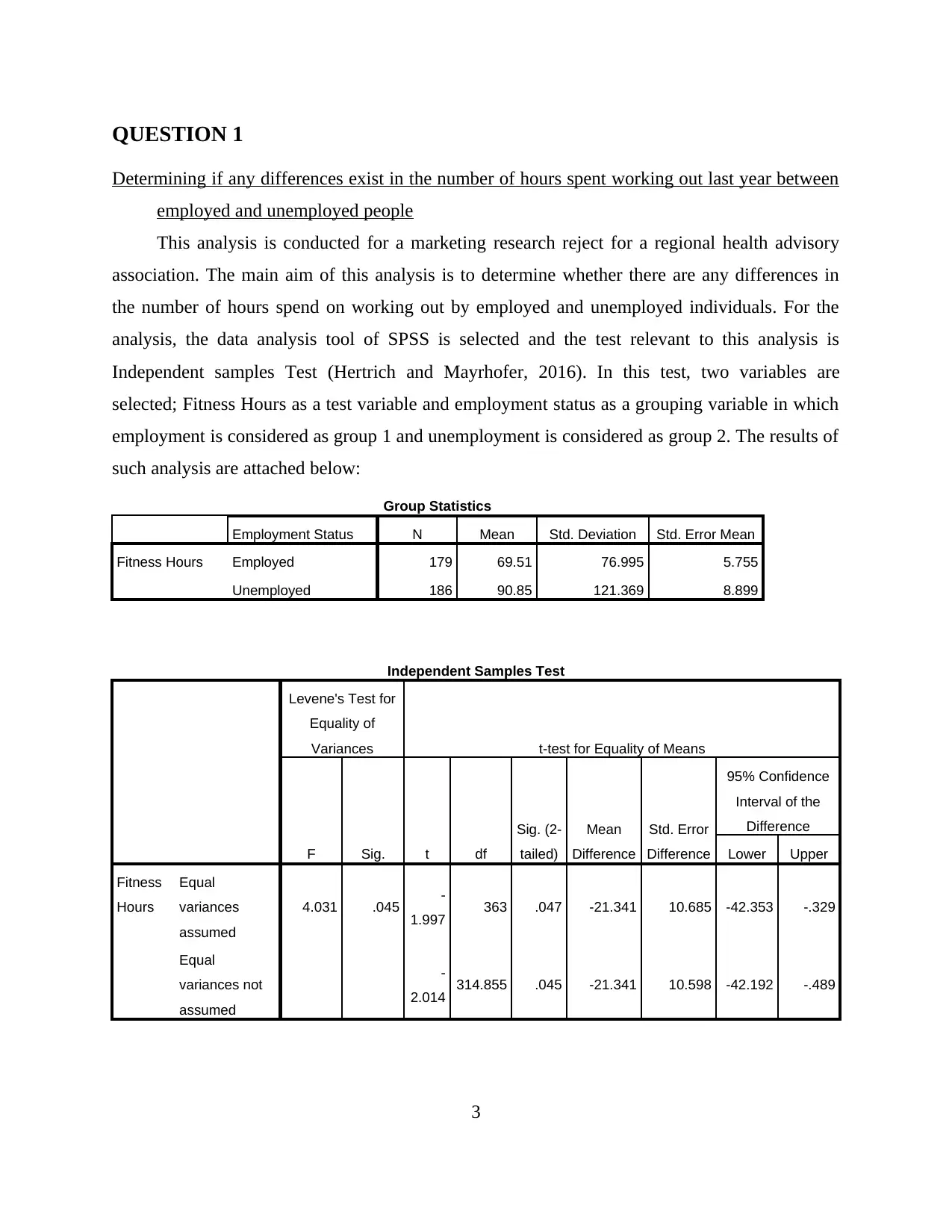
This analysis is conducted for a marketing research reject for a regional health advisory
association. The main aim of this analysis is to determine whether there are any differences in
the number of hours spend on working out by employed and unemployed individuals. For the
analysis, the data analysis tool of SPSS is selected and the test relevant to this analysis is
Independent samples Test (Hertrich and Mayrhofer, 2016). In this test, two variables are
selected; Fitness Hours as a test variable and employment status as a grouping variable in which
employment is considered as group 1 and unemployment is considered as group 2. The results of
such analysis are attached below:
Group Statistics
Employment Status N Mean Std. Deviation Std. Error Mean
Fitness Hours Employed 179 69.51 76.995 5.755
Unemployed 186 90.85 121.369 8.899
Independent Samples Test
Levene's Test for
Equality of
Variances t-test for Equality of Means
F Sig. t df
Sig. (2-
tailed)
Mean
Difference
Std. Error
Difference
95% Confidence
Interval of the
Difference
Lower Upper
Fitness
Hours
Equal
variances
assumed
4.031 .045 -
1.997 363 .047 -21.341 10.685 -42.353 -.329
Equal
variances not
assumed
-
2.014 314.855 .045 -21.341 10.598 -42.192 -.489
3
Determining if any differences exist in the number of hours spent working out last year between
employed and unemployed people
This analysis is conducted for a marketing research reject for a regional health advisory
association. The main aim of this analysis is to determine whether there are any differences in
the number of hours spend on working out by employed and unemployed individuals. For the
analysis, the data analysis tool of SPSS is selected and the test relevant to this analysis is
Independent samples Test (Hertrich and Mayrhofer, 2016). In this test, two variables are
selected; Fitness Hours as a test variable and employment status as a grouping variable in which
employment is considered as group 1 and unemployment is considered as group 2. The results of
such analysis are attached below:
Group Statistics
Employment Status N Mean Std. Deviation Std. Error Mean
Fitness Hours Employed 179 69.51 76.995 5.755
Unemployed 186 90.85 121.369 8.899
Independent Samples Test
Levene's Test for
Equality of
Variances t-test for Equality of Means
F Sig. t df
Sig. (2-
tailed)
Mean
Difference
Std. Error
Difference
95% Confidence
Interval of the
Difference
Lower Upper
Fitness
Hours
Equal
variances
assumed
4.031 .045 -
1.997 363 .047 -21.341 10.685 -42.353 -.329
Equal
variances not
assumed
-
2.014 314.855 .045 -21.341 10.598 -42.192 -.489
3
⊘ This is a preview!⊘
Do you want full access?
Subscribe today to unlock all pages.
Trusted by 1+ million students worldwide
From the above analysis, meaningful insights are gained. In this test assessment, it is
considered that if the significance or p value of the Levene's Test for Equality of Variances is
less than 0.05 then it can be said that there is a significant difference between both the variables.
By observing the above table, it has been seen that p value < 0.05 that is 0.045 which concludes
that the fitness hours of employed individuals are different from the fitness hours of unemployed
people (Arganda-Carreras and et. al., 2017). The above analysis also has a Group statistics table,
from which it has been seen that mean value of employed people is 69.5 which is much lesser
than unemployed people that is 90.85, which implies not only there is statistical significant
difference between employed and unemployed people, the fitness hours of unemployed people
are greater than the fitness hours of employed people.
QUESTION 2
Identifying that whether there an association between total personal income and their spend on
gambling
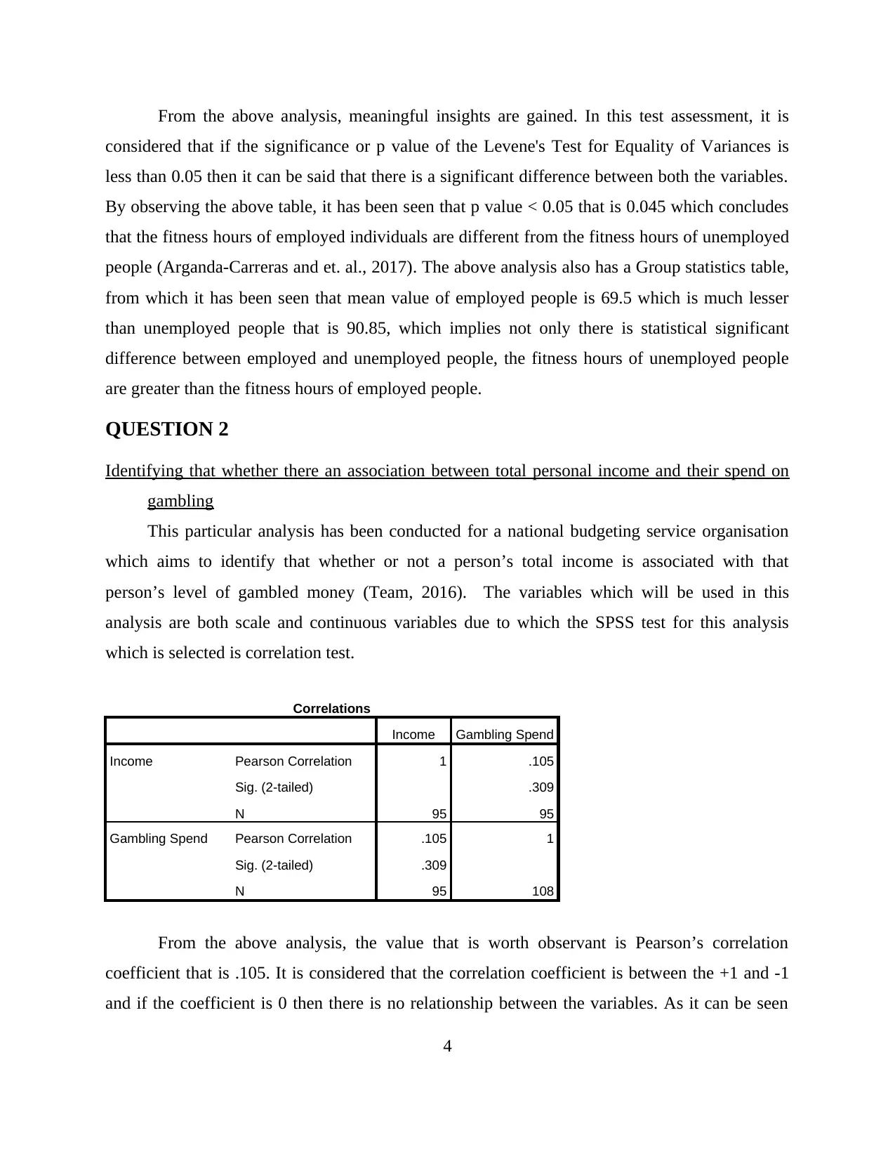
This particular analysis has been conducted for a national budgeting service organisation
which aims to identify that whether or not a person’s total income is associated with that
person’s level of gambled money (Team, 2016). The variables which will be used in this
analysis are both scale and continuous variables due to which the SPSS test for this analysis
which is selected is correlation test.
Correlations
Income Gambling Spend
Income Pearson Correlation 1 .105
Sig. (2-tailed) .309
N 95 95
Gambling Spend Pearson Correlation .105 1
Sig. (2-tailed) .309
N 95 108
From the above analysis, the value that is worth observant is Pearson’s correlation
coefficient that is .105. It is considered that the correlation coefficient is between the +1 and -1
and if the coefficient is 0 then there is no relationship between the variables. As it can be seen
4
considered that if the significance or p value of the Levene's Test for Equality of Variances is
less than 0.05 then it can be said that there is a significant difference between both the variables.
By observing the above table, it has been seen that p value < 0.05 that is 0.045 which concludes
that the fitness hours of employed individuals are different from the fitness hours of unemployed
people (Arganda-Carreras and et. al., 2017). The above analysis also has a Group statistics table,
from which it has been seen that mean value of employed people is 69.5 which is much lesser
than unemployed people that is 90.85, which implies not only there is statistical significant
difference between employed and unemployed people, the fitness hours of unemployed people
are greater than the fitness hours of employed people.
QUESTION 2
Identifying that whether there an association between total personal income and their spend on
gambling
This particular analysis has been conducted for a national budgeting service organisation
which aims to identify that whether or not a person’s total income is associated with that
person’s level of gambled money (Team, 2016). The variables which will be used in this
analysis are both scale and continuous variables due to which the SPSS test for this analysis
which is selected is correlation test.
Correlations
Income Gambling Spend
Income Pearson Correlation 1 .105
Sig. (2-tailed) .309
N 95 95
Gambling Spend Pearson Correlation .105 1
Sig. (2-tailed) .309
N 95 108
From the above analysis, the value that is worth observant is Pearson’s correlation
coefficient that is .105. It is considered that the correlation coefficient is between the +1 and -1
and if the coefficient is 0 then there is no relationship between the variables. As it can be seen
4
Paraphrase This Document
Need a fresh take? Get an instant paraphrase of this document with our AI Paraphraser
that the correlation coefficient is .105, it can be said that there is a weak but positive correlation
between the income of an individual and the money they have spent on gambling. The value of
significance level is more than .05 and that indicates the non significant relationship between
both the variables as the relationship between these variables is weak (Ataman, Kulick and Sim,
2011).
QUESTION 3
Determining the relationship between age and attitude toward gaining a university qualification
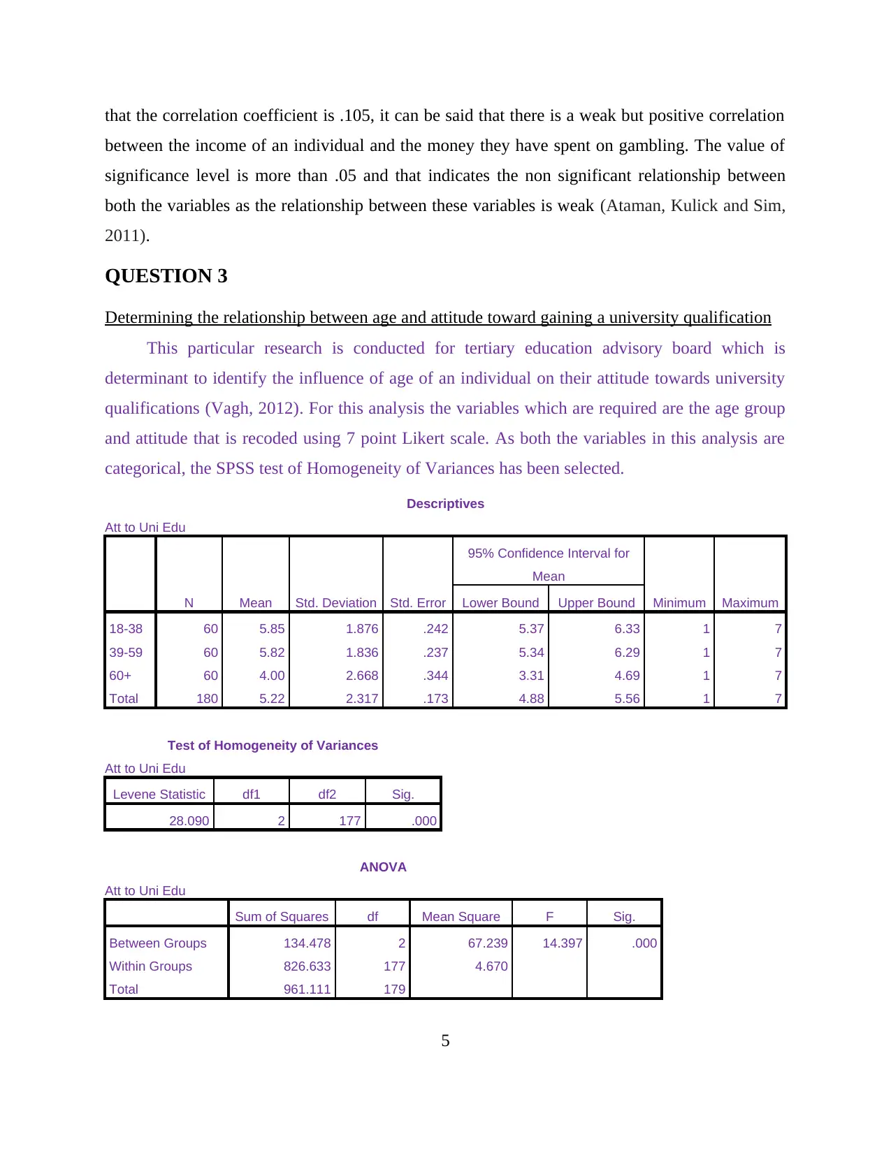
This particular research is conducted for tertiary education advisory board which is
determinant to identify the influence of age of an individual on their attitude towards university
qualifications (Vagh, 2012). For this analysis the variables which are required are the age group
and attitude that is recoded using 7 point Likert scale. As both the variables in this analysis are
categorical, the SPSS test of Homogeneity of Variances has been selected.
Descriptives
Att to Uni Edu
N Mean Std. Deviation Std. Error
95% Confidence Interval for
Mean
Minimum MaximumLower Bound Upper Bound
18-38 60 5.85 1.876 .242 5.37 6.33 1 7
39-59 60 5.82 1.836 .237 5.34 6.29 1 7
60+ 60 4.00 2.668 .344 3.31 4.69 1 7
Total 180 5.22 2.317 .173 4.88 5.56 1 7
Test of Homogeneity of Variances
Att to Uni Edu
Levene Statistic df1 df2 Sig.
28.090 2 177 .000
ANOVA
Att to Uni Edu
Sum of Squares df Mean Square F Sig.
Between Groups 134.478 2 67.239 14.397 .000
Within Groups 826.633 177 4.670
Total 961.111 179
5
between the income of an individual and the money they have spent on gambling. The value of
significance level is more than .05 and that indicates the non significant relationship between
both the variables as the relationship between these variables is weak (Ataman, Kulick and Sim,
2011).
QUESTION 3
Determining the relationship between age and attitude toward gaining a university qualification
This particular research is conducted for tertiary education advisory board which is
determinant to identify the influence of age of an individual on their attitude towards university
qualifications (Vagh, 2012). For this analysis the variables which are required are the age group
and attitude that is recoded using 7 point Likert scale. As both the variables in this analysis are
categorical, the SPSS test of Homogeneity of Variances has been selected.
Descriptives
Att to Uni Edu
N Mean Std. Deviation Std. Error
95% Confidence Interval for
Mean
Minimum MaximumLower Bound Upper Bound
18-38 60 5.85 1.876 .242 5.37 6.33 1 7
39-59 60 5.82 1.836 .237 5.34 6.29 1 7
60+ 60 4.00 2.668 .344 3.31 4.69 1 7
Total 180 5.22 2.317 .173 4.88 5.56 1 7
Test of Homogeneity of Variances
Att to Uni Edu
Levene Statistic df1 df2 Sig.
28.090 2 177 .000
ANOVA
Att to Uni Edu
Sum of Squares df Mean Square F Sig.
Between Groups 134.478 2 67.239 14.397 .000
Within Groups 826.633 177 4.670
Total 961.111 179
5
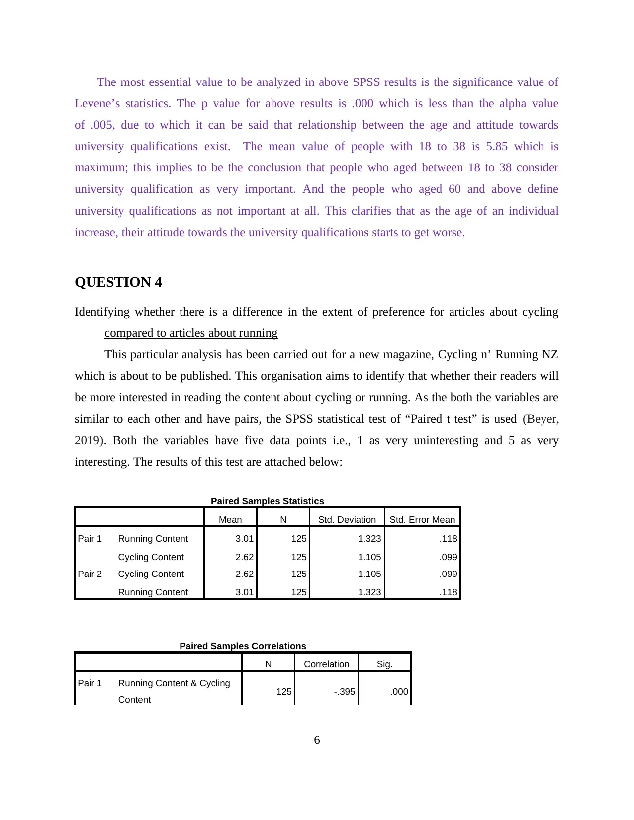
The most essential value to be analyzed in above SPSS results is the significance value of
Levene’s statistics. The p value for above results is .000 which is less than the alpha value
of .005, due to which it can be said that relationship between the age and attitude towards
university qualifications exist. The mean value of people with 18 to 38 is 5.85 which is
maximum; this implies to be the conclusion that people who aged between 18 to 38 consider
university qualification as very important. And the people who aged 60 and above define
university qualifications as not important at all. This clarifies that as the age of an individual
increase, their attitude towards the university qualifications starts to get worse.
QUESTION 4
Identifying whether there is a difference in the extent of preference for articles about cycling
compared to articles about running
This particular analysis has been carried out for a new magazine, Cycling n’ Running NZ
which is about to be published. This organisation aims to identify that whether their readers will
be more interested in reading the content about cycling or running. As the both the variables are
similar to each other and have pairs, the SPSS statistical test of “Paired t test” is used (Beyer,
2019). Both the variables have five data points i.e., 1 as very uninteresting and 5 as very
interesting. The results of this test are attached below:
Paired Samples Statistics
Mean N Std. Deviation Std. Error Mean
Pair 1 Running Content 3.01 125 1.323 .118
Cycling Content 2.62 125 1.105 .099
Pair 2 Cycling Content 2.62 125 1.105 .099
Running Content 3.01 125 1.323 .118
Paired Samples Correlations
N Correlation Sig.
Pair 1 Running Content & Cycling
Content 125 -.395 .000
6
⊘ This is a preview!⊘
Do you want full access?
Subscribe today to unlock all pages.
Trusted by 1+ million students worldwide
Pair 2 Cycling Content & Running
Content 125 -.395 .000
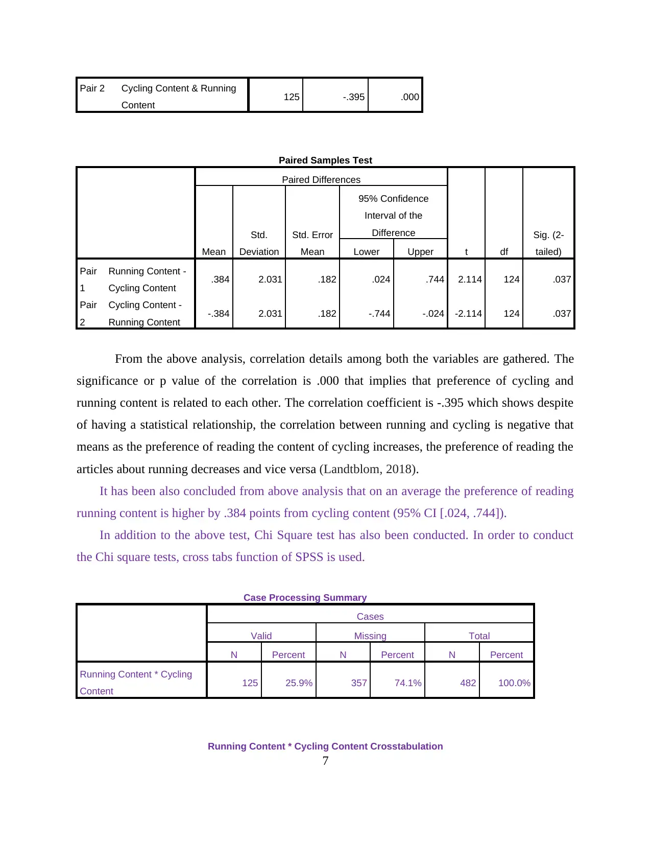
Paired Samples Test
Paired Differences
t df
Sig. (2-
tailed)Mean
Std.
Deviation
Std. Error
Mean
95% Confidence
Interval of the
Difference
Lower Upper
Pair
1
Running Content -
Cycling Content .384 2.031 .182 .024 .744 2.114 124 .037
Pair
2
Cycling Content -
Running Content -.384 2.031 .182 -.744 -.024 -2.114 124 .037
From the above analysis, correlation details among both the variables are gathered. The
significance or p value of the correlation is .000 that implies that preference of cycling and
running content is related to each other. The correlation coefficient is -.395 which shows despite
of having a statistical relationship, the correlation between running and cycling is negative that
means as the preference of reading the content of cycling increases, the preference of reading the
articles about running decreases and vice versa (Landtblom, 2018).
It has been also concluded from above analysis that on an average the preference of reading
running content is higher by .384 points from cycling content (95% CI [.024, .744]).
In addition to the above test, Chi Square test has also been conducted. In order to conduct
the Chi square tests, cross tabs function of SPSS is used.
Case Processing Summary
Cases
Valid Missing Total
N Percent N Percent N Percent
Running Content * Cycling
Content 125 25.9% 357 74.1% 482 100.0%
Running Content * Cycling Content Crosstabulation
7
Content 125 -.395 .000
Paired Samples Test
Paired Differences
t df
Sig. (2-
tailed)Mean
Std.
Deviation
Std. Error
Mean
95% Confidence
Interval of the
Difference
Lower Upper
Pair
1
Running Content -
Cycling Content .384 2.031 .182 .024 .744 2.114 124 .037
Pair
2
Cycling Content -
Running Content -.384 2.031 .182 -.744 -.024 -2.114 124 .037
From the above analysis, correlation details among both the variables are gathered. The
significance or p value of the correlation is .000 that implies that preference of cycling and
running content is related to each other. The correlation coefficient is -.395 which shows despite
of having a statistical relationship, the correlation between running and cycling is negative that
means as the preference of reading the content of cycling increases, the preference of reading the
articles about running decreases and vice versa (Landtblom, 2018).
It has been also concluded from above analysis that on an average the preference of reading
running content is higher by .384 points from cycling content (95% CI [.024, .744]).
In addition to the above test, Chi Square test has also been conducted. In order to conduct
the Chi square tests, cross tabs function of SPSS is used.
Case Processing Summary
Cases
Valid Missing Total
N Percent N Percent N Percent
Running Content * Cycling
Content 125 25.9% 357 74.1% 482 100.0%
Running Content * Cycling Content Crosstabulation
7
Paraphrase This Document
Need a fresh take? Get an instant paraphrase of this document with our AI Paraphraser
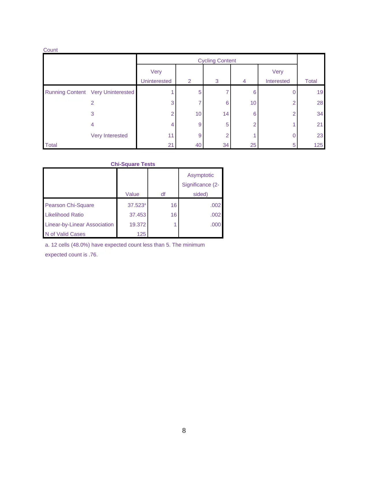
Count
Cycling Content
Total
Very
Uninterested 2 3 4
Very
Interested
Running Content Very Uninterested 1 5 7 6 0 19
2 3 7 6 10 2 28
3 2 10 14 6 2 34
4 4 9 5 2 1 21
Very Interested 11 9 2 1 0 23
Total 21 40 34 25 5 125
Chi-Square Tests
Value df
Asymptotic
Significance (2-
sided)
Pearson Chi-Square 37.523a 16 .002
Likelihood Ratio 37.453 16 .002
Linear-by-Linear Association 19.372 1 .000
N of Valid Cases 125
a. 12 cells (48.0%) have expected count less than 5. The minimum
expected count is .76.
8
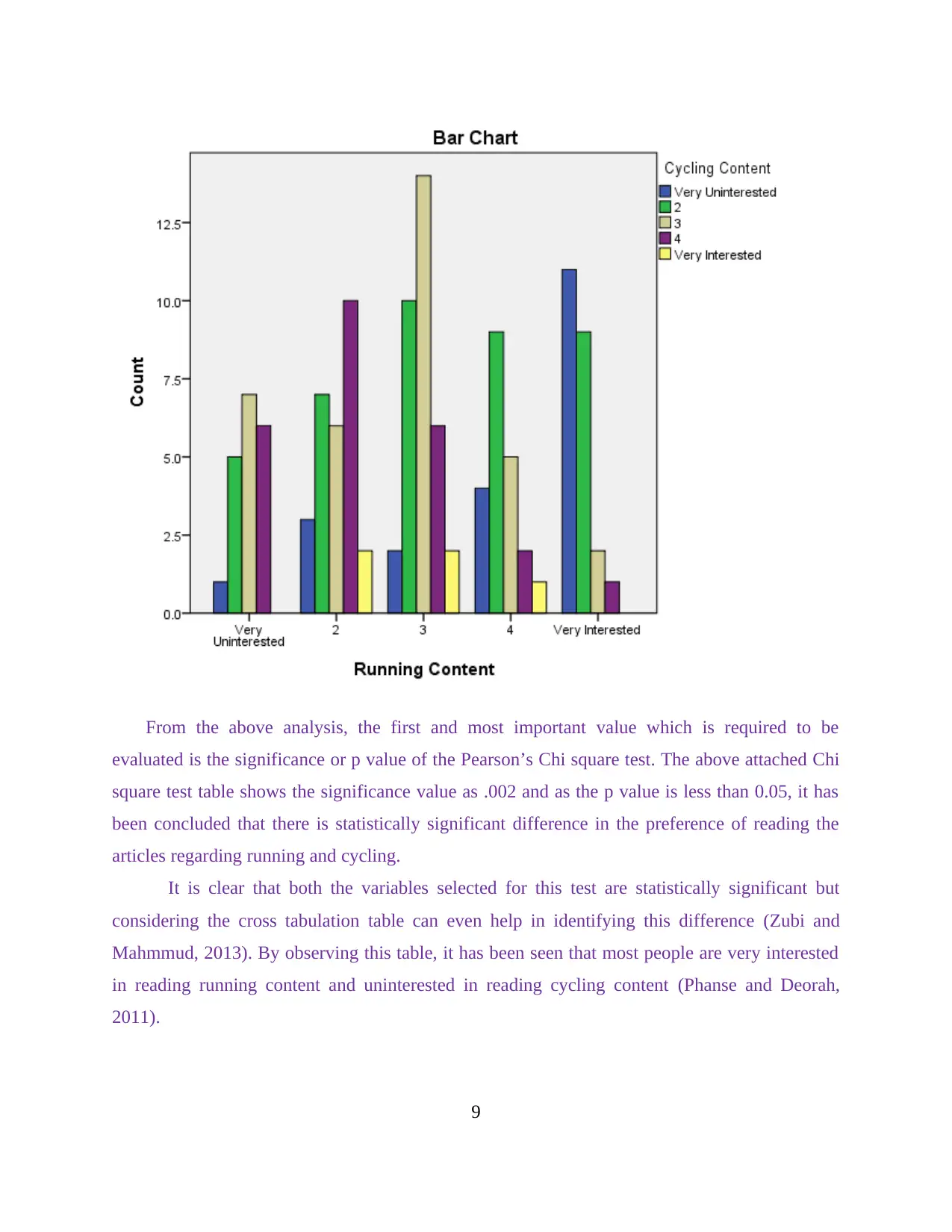
From the above analysis, the first and most important value which is required to be
evaluated is the significance or p value of the Pearson’s Chi square test. The above attached Chi
square test table shows the significance value as .002 and as the p value is less than 0.05, it has
been concluded that there is statistically significant difference in the preference of reading the
articles regarding running and cycling.
It is clear that both the variables selected for this test are statistically significant but
considering the cross tabulation table can even help in identifying this difference (Zubi and
Mahmmud, 2013). By observing this table, it has been seen that most people are very interested
in reading running content and uninterested in reading cycling content (Phanse and Deorah,
2011).
9
⊘ This is a preview!⊘
Do you want full access?
Subscribe today to unlock all pages.
Trusted by 1+ million students worldwide
QUESTION 5
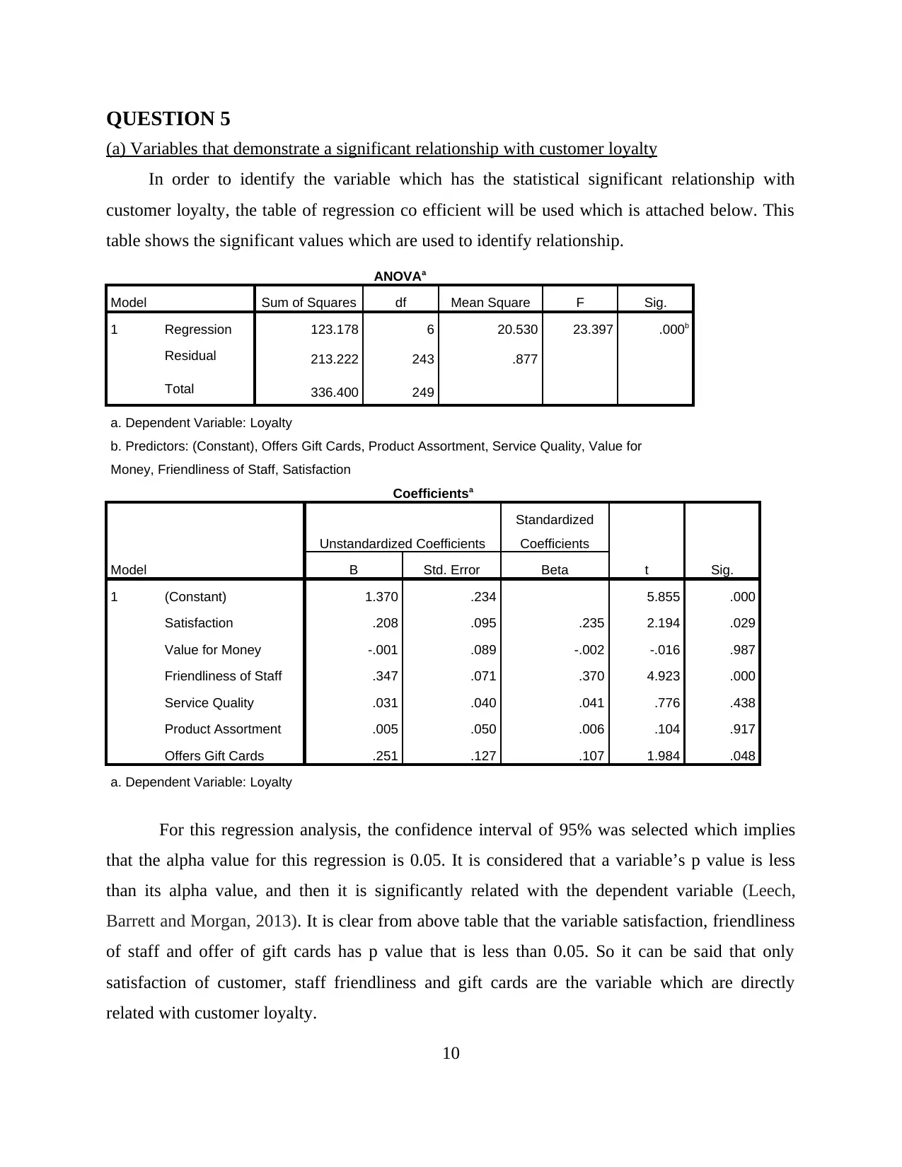
(a) Variables that demonstrate a significant relationship with customer loyalty
In order to identify the variable which has the statistical significant relationship with
customer loyalty, the table of regression co efficient will be used which is attached below. This
table shows the significant values which are used to identify relationship.
ANOVAa
Model Sum of Squares df Mean Square F Sig.
1 Regression 123.178 6 20.530 23.397 .000b
Residual 213.222 243 .877
Total 336.400 249
a. Dependent Variable: Loyalty
b. Predictors: (Constant), Offers Gift Cards, Product Assortment, Service Quality, Value for
Money, Friendliness of Staff, Satisfaction
Coefficientsa
Model
Unstandardized Coefficients
Standardized
Coefficients
t Sig.B Std. Error Beta
1 (Constant) 1.370 .234 5.855 .000
Satisfaction .208 .095 .235 2.194 .029
Value for Money -.001 .089 -.002 -.016 .987
Friendliness of Staff .347 .071 .370 4.923 .000
Service Quality .031 .040 .041 .776 .438
Product Assortment .005 .050 .006 .104 .917
Offers Gift Cards .251 .127 .107 1.984 .048
a. Dependent Variable: Loyalty
For this regression analysis, the confidence interval of 95% was selected which implies
that the alpha value for this regression is 0.05. It is considered that a variable’s p value is less
than its alpha value, and then it is significantly related with the dependent variable (Leech,
Barrett and Morgan, 2013). It is clear from above table that the variable satisfaction, friendliness
of staff and offer of gift cards has p value that is less than 0.05. So it can be said that only
satisfaction of customer, staff friendliness and gift cards are the variable which are directly
related with customer loyalty.
10
Paraphrase This Document
Need a fresh take? Get an instant paraphrase of this document with our AI Paraphraser
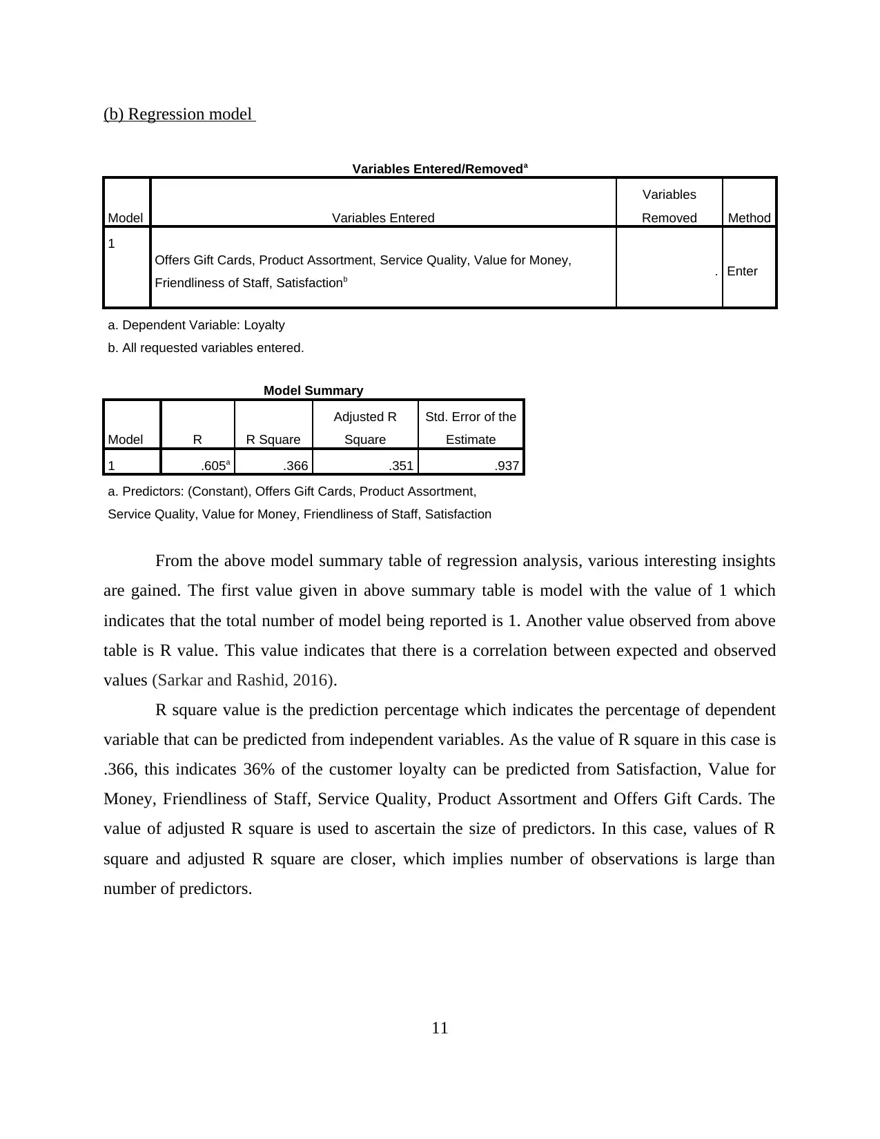
(b) Regression model
Variables Entered/Removeda
Model Variables Entered
Variables
Removed Method
1
Offers Gift Cards, Product Assortment, Service Quality, Value for Money,
Friendliness of Staff, Satisfactionb . Enter
a. Dependent Variable: Loyalty
b. All requested variables entered.
Model Summary
Model R R Square
Adjusted R
Square
Std. Error of the
Estimate
1 .605a .366 .351 .937
a. Predictors: (Constant), Offers Gift Cards, Product Assortment,
Service Quality, Value for Money, Friendliness of Staff, Satisfaction
From the above model summary table of regression analysis, various interesting insights
are gained. The first value given in above summary table is model with the value of 1 which
indicates that the total number of model being reported is 1. Another value observed from above
table is R value. This value indicates that there is a correlation between expected and observed
values (Sarkar and Rashid, 2016).
R square value is the prediction percentage which indicates the percentage of dependent
variable that can be predicted from independent variables. As the value of R square in this case is
.366, this indicates 36% of the customer loyalty can be predicted from Satisfaction, Value for
Money, Friendliness of Staff, Service Quality, Product Assortment and Offers Gift Cards. The
value of adjusted R square is used to ascertain the size of predictors. In this case, values of R
square and adjusted R square are closer, which implies number of observations is large than
number of predictors.
11
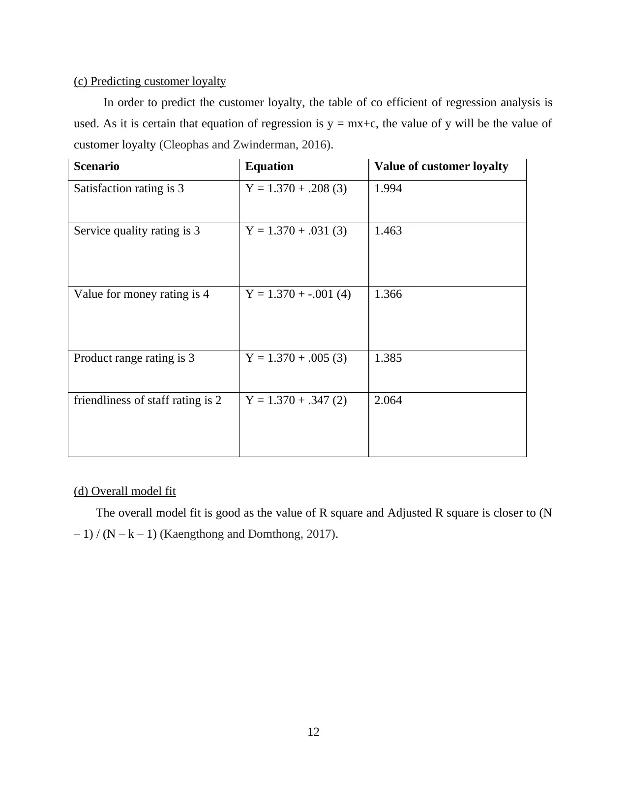
(c) Predicting customer loyalty
In order to predict the customer loyalty, the table of co efficient of regression analysis is
used. As it is certain that equation of regression is y = mx+c, the value of y will be the value of
customer loyalty (Cleophas and Zwinderman, 2016).
Scenario Equation Value of customer loyalty
Satisfaction rating is 3 Y = 1.370 + .208 (3) 1.994
Service quality rating is 3 Y = 1.370 + .031 (3) 1.463
Value for money rating is 4 Y = 1.370 + -.001 (4) 1.366
Product range rating is 3 Y = 1.370 + .005 (3) 1.385
friendliness of staff rating is 2 Y = 1.370 + .347 (2) 2.064
(d) Overall model fit
The overall model fit is good as the value of R square and Adjusted R square is closer to (N
– 1) / (N – k – 1) (Kaengthong and Domthong, 2017).
12
⊘ This is a preview!⊘
Do you want full access?
Subscribe today to unlock all pages.
Trusted by 1+ million students worldwide
1 out of 13
Related Documents


Your All-in-One AI-Powered Toolkit for Academic Success.
+13062052269
info@desklib.com
Available 24*7 on WhatsApp / Email
![[object Object]](/_next/static/media/star-bottom.7253800d.svg)
Unlock your academic potential
Copyright © 2020–2026 A2Z Services. All Rights Reserved. Developed and managed by ZUCOL.