Markov Chains, Orthogonal Projections: Complete Homework Solution
VerifiedAdded on 2023/03/21
|18
|4339
|47
Homework Assignment
AI Summary
This assignment solution covers two main topics: Markov Chains and Orthogonal Projections. The Markov Chains section involves constructing and analyzing a transition matrix for a warehouse inventory system, determining the week-by-week succession of system states using matrix multiplication, and finding the steady-state vector. The Orthogonal Projections section focuses on finding curves of best fit for given data points, including determining parabolas and linear combinations of sine and cosine waves that satisfy specific data points. The solution demonstrates the application of matrix operations, Gaussian elimination, and quadratic formulas to solve problems related to Markov Chains and curve fitting using orthogonal projections.

Part A: Introduction to Markov Chains
Markov Chains are a useful matrix-based technique that is widely used in modern
probability theory. Here’s the basic idea: Suppose the components of a system can exist
in number of physical states {s1,….,sn} The components of the system will begin in one
of these states, and then successively move from one state to the next with a certain
probability. Each move (or "transition") is called a step. Suppose a component is
currently in state si, and then it moves to state sj at the next step with a probability
denoted by pij. If this probability depends only on the current state, and not on any
previous state of the system, then pij is referred to as a transition probability, and the
succession of discrete states of the system as it evolves over time is known as a Markov
chain.
Transition probabilities can be used to construct a Markov matrix. A Markov matrix has
two key properties: every entry of the matrix of non-negative (such a matrix is said to be
"regular"); and every column of the matrix adds to 1.
Consider the following definitions and theorems relevant to the theory of Markov Chains,
and then answer the questions that follow:
Paraphrase This Document
Need a fresh take? Get an instant paraphrase of this document with our AI Paraphraser
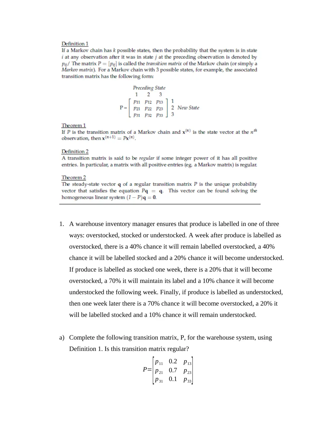
1. A warehouse inventory manager ensures that produce is labelled in one of three
ways: overstocked, stocked or understocked. A week after produce is labelled as
overstocked, there is a 40% chance it will remain labelled overstocked, a 40%
chance it will be labelled stocked and a 20% chance it will become understocked.
If produce is labelled as stocked one week, there is a 20% that it will become
overstocked, a 70% it will maintain its label and a 10% chance it will become
understocked the following week. Finally, if produce is labelled as understocked,
then one week later there is a 70% chance it will become overstocked, a 20% it
will be labelled stocked and a 10% chance it will remain understocked.
a) Complete the following transition matrix, P, for the warehouse system, using
Definition 1. Is this transition matrix regular?
P=
[ p11 0.2 p13
p21 0.7 p23
p31 0.1 p33 ]
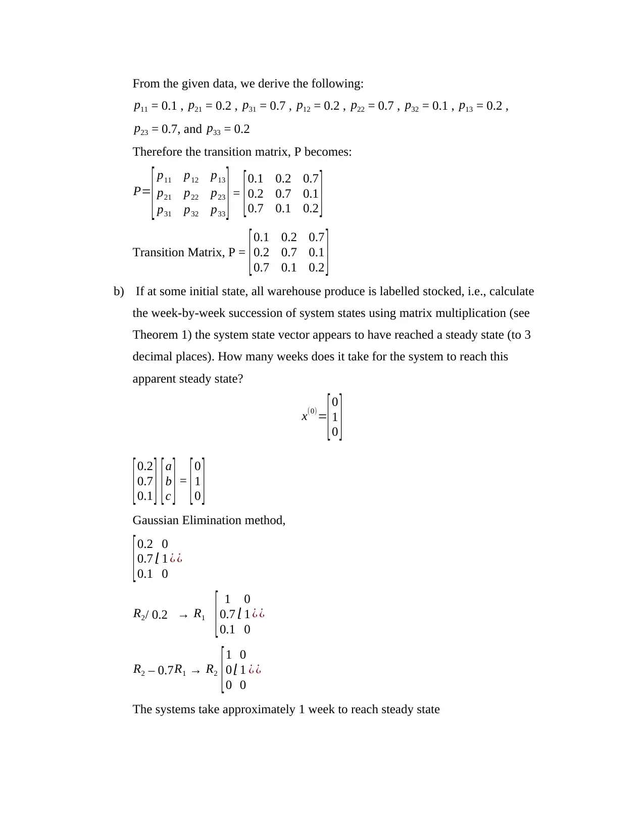
From the given data, we derive the following:
p11 = 0.1 , p21 = 0.2 , p31 = 0.7 , p12 = 0.2 , p22 = 0.7 , p32 = 0.1 , p13 = 0.2 ,
p23 = 0.7, and p33 = 0.2
Therefore the transition matrix, P becomes:
P=
[ p11 p12 p13
p21 p22 p23
p31 p32 p33 ] = [0.1 0.2 0.7
0.2 0.7 0.1
0.7 0.1 0.2 ]
Transition Matrix, P = [0.1 0.2 0.7
0.2 0.7 0.1
0.7 0.1 0.2 ]
b) If at some initial state, all warehouse produce is labelled stocked, i.e., calculate
the week-by-week succession of system states using matrix multiplication (see
Theorem 1) the system state vector appears to have reached a steady state (to 3
decimal places). How many weeks does it take for the system to reach this
apparent steady state?
x(0)=
[ 0
1
0 ]
[0.2
0.7
0.1 ] [a
b
c ] = [ 0
1
0 ]
Gaussian Elimination method,
[0.2
0.7
0.1
⌊
0
1
0
¿ ¿
R2/ 0.2 → R1
[ 1
0.7
0.1
⌊
0
1
0
¿ ¿
R2 – 0.7 R1 → R2
[ 1
0
0
⌊
0
1
0
¿ ¿
The systems take approximately 1 week to reach steady state
⊘ This is a preview!⊘
Do you want full access?
Subscribe today to unlock all pages.
Trusted by 1+ million students worldwide
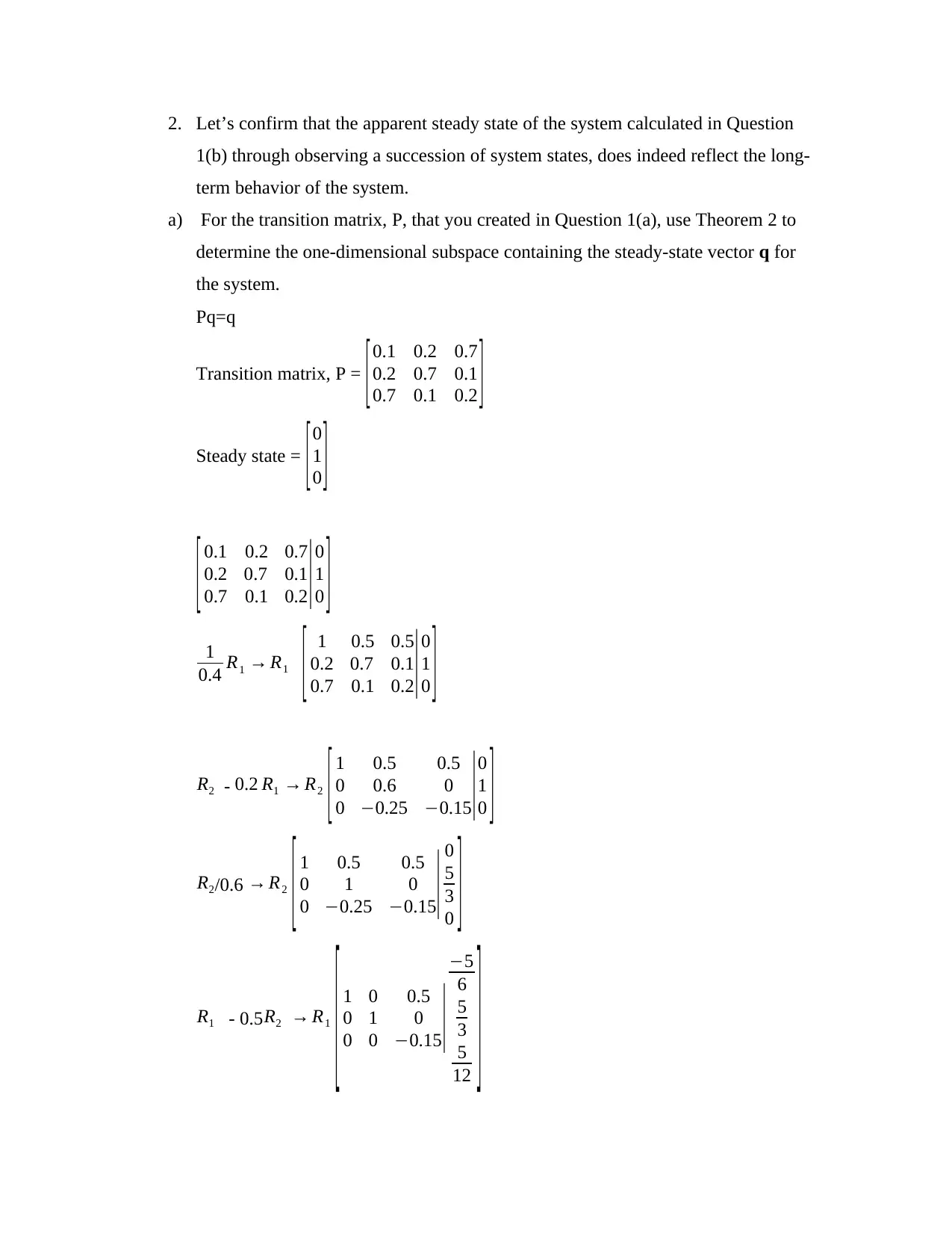
2. Let’s confirm that the apparent steady state of the system calculated in Question
1(b) through observing a succession of system states, does indeed reflect the long-
term behavior of the system.
a) For the transition matrix, P, that you created in Question 1(a), use Theorem 2 to
determine the one-dimensional subspace containing the steady-state vector q for
the system.
Pq=q
Transition matrix, P = [0.1 0.2 0.7
0.2 0.7 0.1
0.7 0.1 0.2 ]
Steady state = [ 0
1
0 ]
[ 0.1 0.2 0.7
0.2 0.7 0.1
0.7 0.1 0.2| 0
1
0 ]
1
0.4 R1 → R1
[ 1 0.5 0.5
0.2 0.7 0.1
0.7 0.1 0.2|0
1
0 ]
R2 - 0.2 R1 → R2
[ 1 0.5 0.5
0 0.6 0
0 −0.25 −0.15|
0
1
0 ]
R2/0.6 → R2
[ 1 0.5 0.5
0 1 0
0 −0.25 −0.15| 0
5
3
0 ]
R1 - 0.5R2 → R1
[ 1 0 0.5
0 1 0
0 0 −0.15|
−5
6
5
3
5
12 ]
Paraphrase This Document
Need a fresh take? Get an instant paraphrase of this document with our AI Paraphraser
R3/-0.15 → R3
[ 1 0 0.5
0 1 0
0 0 1 |
−5
6
5
3
−25
9
]
R1 - 0.5R3 → R1
[ 1 0 0
0 1 0
0 0 1|
5
9
5
3
−25
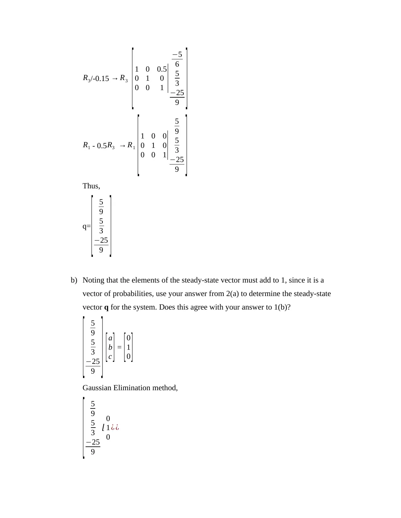
9 ]Thus,
q=
[ 5
9
5
3
−25
9 ]
b) Noting that the elements of the steady-state vector must add to 1, since it is a
vector of probabilities, use your answer from 2(a) to determine the steady-state
vector q for the system. Does this agree with your answer to 1(b)?
[ 5
9
5
3
−25
9 ] [ a
b
c ] = [0
1
0 ]
Gaussian Elimination method,
[ 5
9
5
3
−25
9
⌊
0
1
0
¿ ¿
[ 1 0 0.5
0 1 0
0 0 1 |
−5
6
5
3
−25
9
]
R1 - 0.5R3 → R1
[ 1 0 0
0 1 0
0 0 1|
5
9
5
3
−25
9 ]Thus,
q=
[ 5
9
5
3
−25
9 ]
b) Noting that the elements of the steady-state vector must add to 1, since it is a
vector of probabilities, use your answer from 2(a) to determine the steady-state
vector q for the system. Does this agree with your answer to 1(b)?
[ 5
9
5
3
−25
9 ] [ a
b
c ] = [0
1
0 ]
Gaussian Elimination method,
[ 5
9
5
3
−25
9
⌊
0
1
0
¿ ¿
R1/(5/9) → R1
[ 1
5
3
−25
9
⌊
0
1
0
¿ ¿
R2 – 5/3 R1 → R2
[1
0
0
⌊
0
1
0
¿ ¿
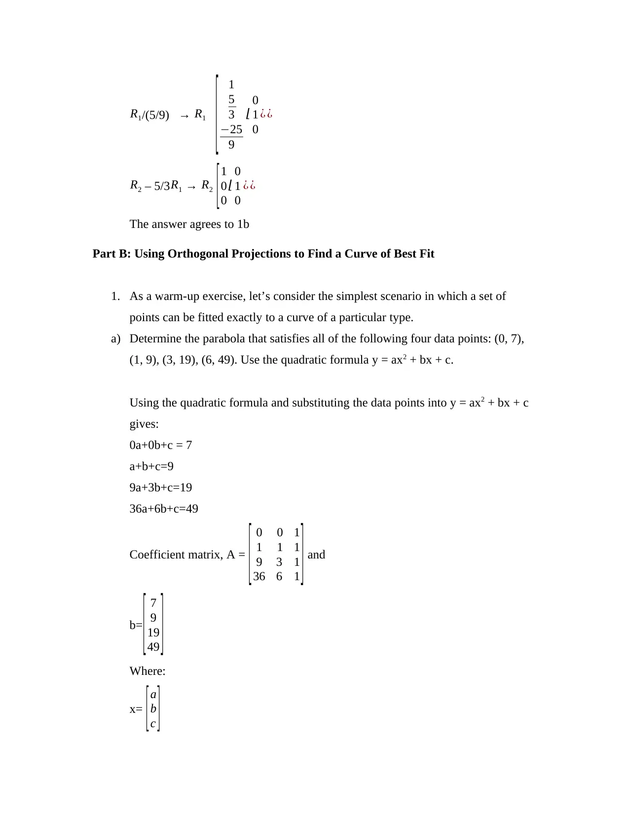
The answer agrees to 1b
Part B: Using Orthogonal Projections to Find a Curve of Best Fit
1. As a warm-up exercise, let’s consider the simplest scenario in which a set of
points can be fitted exactly to a curve of a particular type.
a) Determine the parabola that satisfies all of the following four data points: (0, 7),
(1, 9), (3, 19), (6, 49). Use the quadratic formula y = ax2 + bx + c.
Using the quadratic formula and substituting the data points into y = ax2 + bx + c
gives:
0a+0b+c = 7
a+b+c=9
9a+3b+c=19
36a+6b+c=49
Coefficient matrix, A =
[ 0 0 1
1 1 1
9 3 1
36 6 1 ] and
b=
[ 7
9
19
49 ]
Where:
x= [ a
b
c ]
[ 1
5
3
−25
9
⌊
0
1
0
¿ ¿
R2 – 5/3 R1 → R2
[1
0
0
⌊
0
1
0
¿ ¿
The answer agrees to 1b
Part B: Using Orthogonal Projections to Find a Curve of Best Fit
1. As a warm-up exercise, let’s consider the simplest scenario in which a set of
points can be fitted exactly to a curve of a particular type.
a) Determine the parabola that satisfies all of the following four data points: (0, 7),
(1, 9), (3, 19), (6, 49). Use the quadratic formula y = ax2 + bx + c.
Using the quadratic formula and substituting the data points into y = ax2 + bx + c
gives:
0a+0b+c = 7
a+b+c=9
9a+3b+c=19
36a+6b+c=49
Coefficient matrix, A =
[ 0 0 1
1 1 1
9 3 1
36 6 1 ] and
b=
[ 7
9
19
49 ]
Where:
x= [ a
b
c ]
⊘ This is a preview!⊘
Do you want full access?
Subscribe today to unlock all pages.
Trusted by 1+ million students worldwide
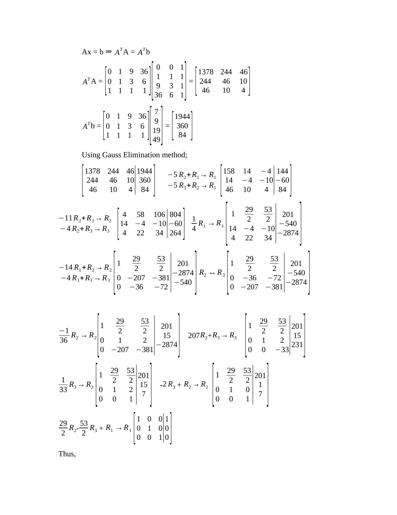
Ax = b ⇒ AT A = AT b
AT A = [0 1 9 36
0 1 3 6
1 1 1 1 ] [ 0 0 1
1 1 1
9 3 1
36 6 1 ] = [1378 244 46
244 46 10
46 10 4 ]
AT b = [0 1 9 36
0 1 3 6
1 1 1 1 ] [ 7
9
19
49 ] = [1944
360
84 ]
Using Gauss Elimination method;
[ 1378 244 46
244 46 10
46 10 4 |
1944
360
84 ] −5 R2 + R1 → R1
−5 R3 + R2 → R1 [ 158 14 −4
14 −4 −10
46 10 4 | 144
−60
84 ]
−11 R2+ R1 → R2
−4 R2 +R3 → R3 [ 4 58 106
14 −4 −10
4 22 34 | 804
−60
264 ] 1
4 R1 → R1
[ 1 29
2
53
2
14 −4 −10
4 22 34 | 201
−540
−2874 ]
−14 R1 +R2 → R2
−4 R1+R3 → R3 [ 1 29
2
53
2
0 −207 −381
0 −36 −72 | 201
−2874
−540 ] R2 ↔ R3
[ 1 29
2
53
2
0 −36 −72
0 −207 −381
| 201
−540
−2874 ]
−1
36 R2 → R2
[ 1 29
2
53
2
0 1 2
0 −207 −381
| 201
15
−2874 ] 207R2+R3 → R3
[ 1 29
2
53
2
0 1 2
0 0 −33
|201
15
231 ]
1
33 R3 → R3
[ 1 29
2
53
2
0 1 2
0 0 1 |201
15
7 ] -2 R3 + R2 → R2
[ 1 29
2
53
2
0 1 0
0 0 1 |201
1
7 ]
29
2 R2- 53
2 R3 + R1 → R1
[ 1 0 0
0 1 0
0 0 1|
1
0
0 ]
Thus,
Paraphrase This Document
Need a fresh take? Get an instant paraphrase of this document with our AI Paraphraser
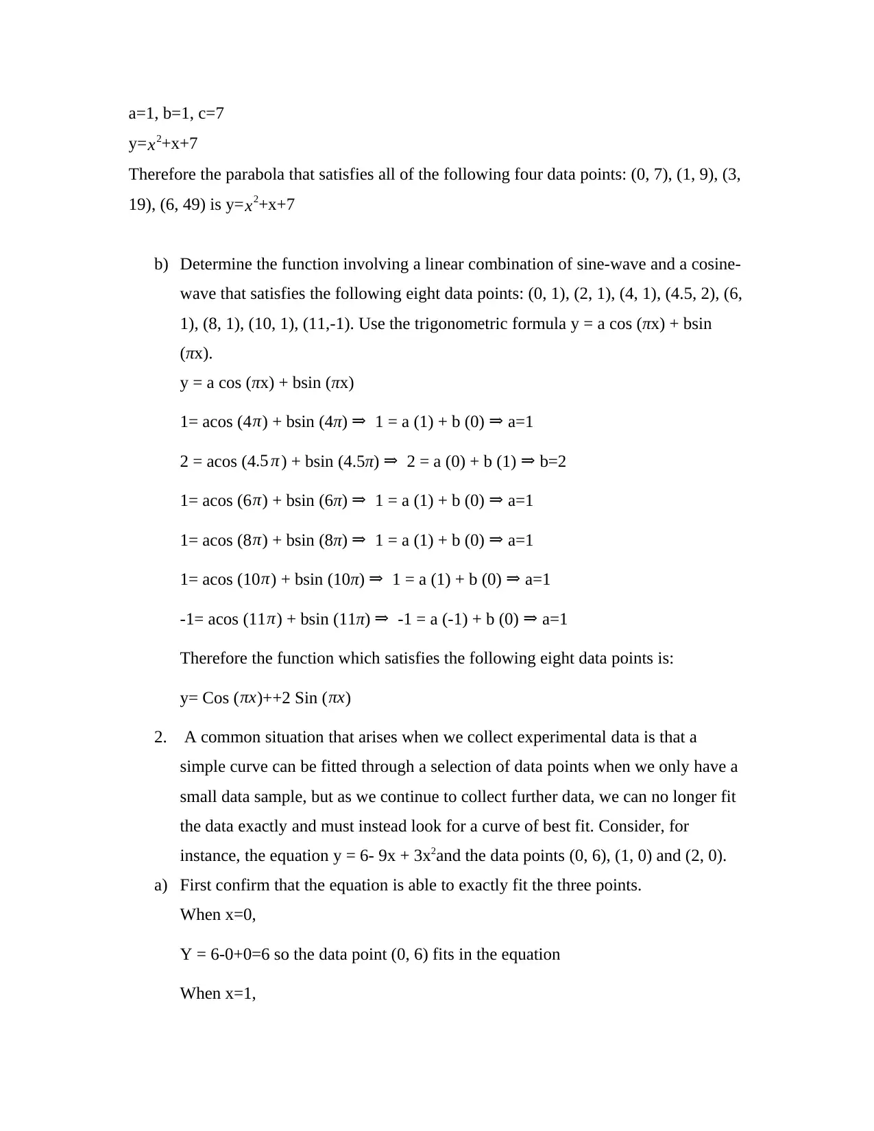
a=1, b=1, c=7
y=x2+x+7
Therefore the parabola that satisfies all of the following four data points: (0, 7), (1, 9), (3,
19), (6, 49) is y= x2+x+7
b) Determine the function involving a linear combination of sine-wave and a cosine-
wave that satisfies the following eight data points: (0, 1), (2, 1), (4, 1), (4.5, 2), (6,
1), (8, 1), (10, 1), (11,-1). Use the trigonometric formula y = a cos (πx) + bsin
(πx).
y = a cos (πx) + bsin (πx)
1= acos (4 π) + bsin (4π) ⇒ 1 = a (1) + b (0) ⇒ a=1
2 = acos (4.5 π ) + bsin (4.5π) ⇒ 2 = a (0) + b (1) ⇒ b=2
1= acos (6 π) + bsin (6π) ⇒ 1 = a (1) + b (0) ⇒ a=1
1= acos (8 π) + bsin (8π) ⇒ 1 = a (1) + b (0) ⇒ a=1
1= acos (10 π) + bsin (10π) ⇒ 1 = a (1) + b (0) ⇒ a=1
-1= acos (11 π) + bsin (11π) ⇒ -1 = a (-1) + b (0) ⇒ a=1
Therefore the function which satisfies the following eight data points is:
y= Cos (πx)++2 Sin (πx)
2. A common situation that arises when we collect experimental data is that a
simple curve can be fitted through a selection of data points when we only have a
small data sample, but as we continue to collect further data, we can no longer fit
the data exactly and must instead look for a curve of best fit. Consider, for
instance, the equation y = 6- 9x + 3x2and the data points (0, 6), (1, 0) and (2, 0).
a) First confirm that the equation is able to exactly fit the three points.
When x=0,
Y = 6-0+0=6 so the data point (0, 6) fits in the equation
When x=1,

Y = 6-9+3=0 so the data point (1, 0) fits in the equation
When x=2,
Y = 6-18+12=0 so the data point (2, 0) fits in the equation
Therefore the equation y = 6- 9x + 3x2 exactly fit the three points (0, 6), (1, 0) and
(2, 0).
b) Suppose we now collect some additional data. If the data point (3, 4) is added to
the above data, show that the equation above can no longer exactly fit all four data
points.
When x=3,
y = 6- 9(3) + 3(32) = 6
Therefore (3, 4) does not lie on the equation y = 6- 9x + 3x2
c) Using the quadratic formula from Question 1(a) above, find the parabola of best
fit for the set of four data points.
Using the quadratic formula and substituting the data points into y = ax2 + bx + c
gives:
Let y = a + bx+ c x2
6= 1a + 0b +0c
0= 1a + 1b +1c
0 = 1a + 2b +4c
4= 1a + 3b +9c
Coefficient matrix, A =
[1 0 1
1 1 1
1 2 4
1 3 9 ] and
b=
[6
0
0
4 ]
Where:
⊘ This is a preview!⊘
Do you want full access?
Subscribe today to unlock all pages.
Trusted by 1+ million students worldwide
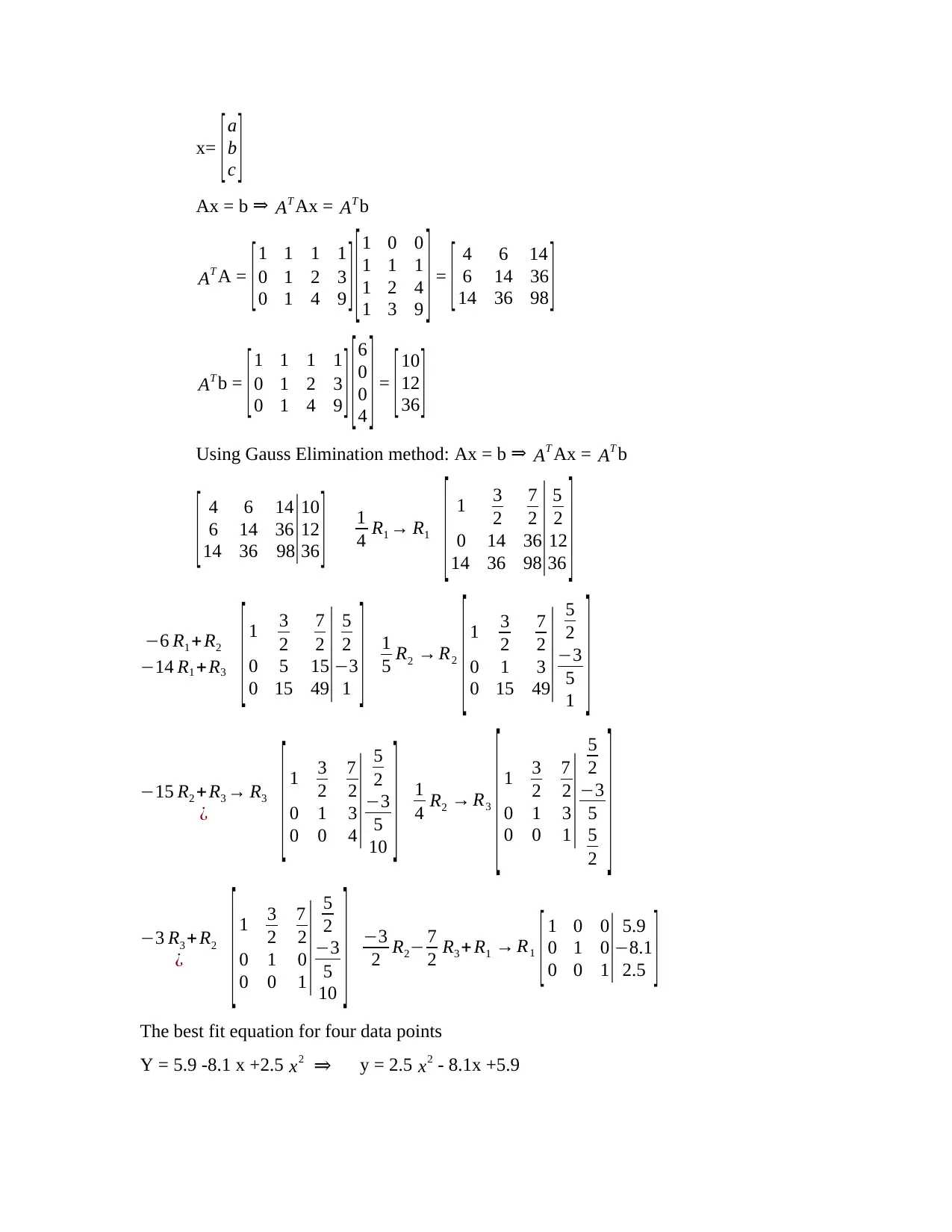
x= [ a
b
c ]
Ax = b ⇒ AT Ax = AT b
AT A = [ 1 1 1 1
0 1 2 3
0 1 4 9 ] [ 1 0 0
1 1 1
1 2 4
1 3 9 ] = [ 4 6 14
6 14 36
14 36 98 ]
AT b = [1 1 1 1
0 1 2 3
0 1 4 9 ] [6
0
0
4 ] = [10
12
36 ]
Using Gauss Elimination method: Ax = b ⇒ AT Ax = AT b
[ 4 6 14
6 14 36
14 36 98|
10
12
36 ] 1
4 R1 → R1
[ 1 3
2
7
2
0 14 36
14 36 98
| 5
2
12
36 ]
−6 R1 +R2
−14 R1 +R3 [ 1 3
2
7
2
0 5 15
0 15 49
| 5
2
−3
1 ] 1
5 R2 → R2
[ 1 3
2
7
2
0 1 3
0 15 49
| 5
2
−3
5
1 ]
−15 R2 + R3 → R3
¿ [ 1 3
2
7
2
0 1 3
0 0 4 | 5
2
−3
5
10 ] 1
4 R2 → R3
[ 1 3
2
7
2
0 1 3
0 0 1 | 5
2
−3
5
5
2 ]
−3 R3 + R2
¿ [ 1 3
2
7
2
0 1 0
0 0 1
| 5
2
−3
5
10 ] −3
2 R2− 7
2 R3 + R1 → R1
[ 1 0 0
0 1 0
0 0 1| 5.9
−8.1
2.5 ]
The best fit equation for four data points
Y = 5.9 -8.1 x +2.5 x2 ⇒ y = 2.5 x2 - 8.1x +5.9
Paraphrase This Document
Need a fresh take? Get an instant paraphrase of this document with our AI Paraphraser
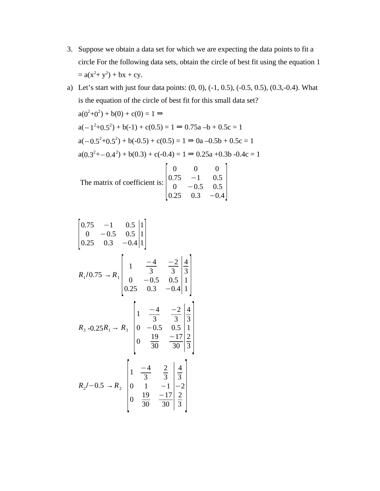
3. Suppose we obtain a data set for which we are expecting the data points to fit a
circle For the following data sets, obtain the circle of best fit using the equation 1
= a(x2+ y2) + bx + cy.
a) Let’s start with just four data points: (0, 0), (-1, 0.5), (-0.5, 0.5), (0.3,-0.4). What
is the equation of the circle of best fit for this small data set?
a(02+02) + b(0) + c(0) = 1 ⇒
a( −12+0.52) + b(-1) + c(0.5) = 1 ⇒ 0.75a –b + 0.5c = 1
a(−0.52+0.52) + b(-0.5) + c(0.5) = 1 ⇒ 0a –0.5b + 0.5c = 1
a( 0.32+−0.42) + b(0.3) + c(-0.4) = 1 ⇒ 0.25a +0.3b -0.4c = 1
The matrix of coefficient is:
[ 0 0 0
0.75 −1 0.5
0 −0.5 0.5
0.25 0.3 −0.4 ]
[ 0.75 −1 0.5
0 −0.5 0.5
0.25 0.3 −0.4 |
1
1
1 ]
R1 /0.75 → R1
[ 1 −4
3
−2
3
0 −0.5 0.5
0.25 0.3 −0.4
| 4
3
1
1 ]
R3 -0.25 R1 → R3
[1 −4
3
−2
3
0 −0.5 0.5
0 19
30
−17
30 | 4
3
1
2
3 ]
R2 /−0.5 → R2
[ 1 −4
3
2
3
0 1 −1
0 19
30
−17
30 | 4
3
−2
2
3 ]
R1+ 4
3 R3 → R1
[ 1 0 −2
3
0 1 −1
0 0 1
15 |
−4
3
−2
29
15 ]
R3 /15 → R3
[1 0 −2
3
0 1 −1
0 0 1 |−4
3
−2
29 ]
R1+ 2
3 R3 → R1
[ 1 0 0
0 1 0
0 0 1 |
18
27
29 ]
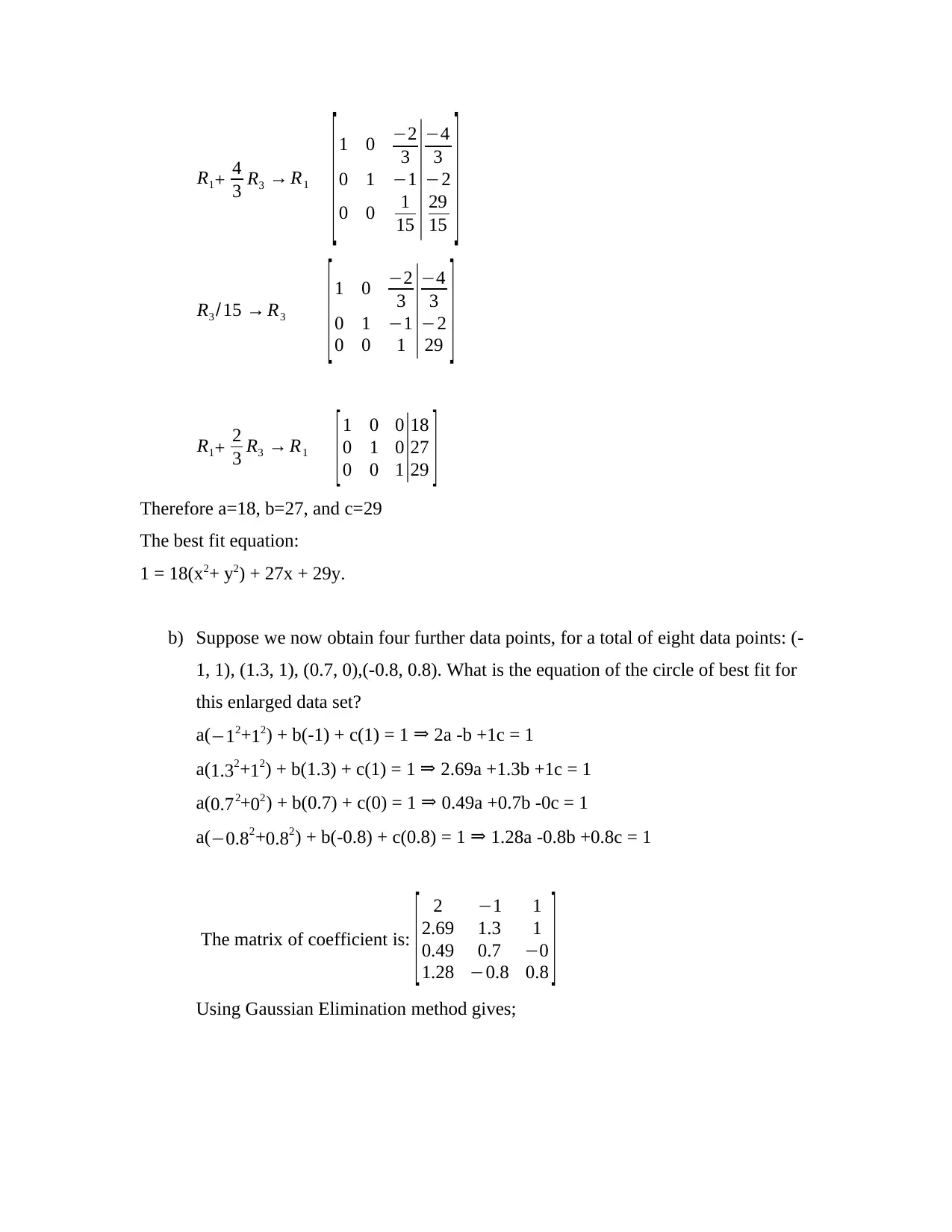
Therefore a=18, b=27, and c=29
The best fit equation:
1 = 18(x2+ y2) + 27x + 29y.
b) Suppose we now obtain four further data points, for a total of eight data points: (-
1, 1), (1.3, 1), (0.7, 0),(-0.8, 0.8). What is the equation of the circle of best fit for
this enlarged data set?
a( −12+12) + b(-1) + c(1) = 1 ⇒ 2a -b +1c = 1
a(1.32+12) + b(1.3) + c(1) = 1 ⇒ 2.69a +1.3b +1c = 1
a( 0.72+02) + b(0.7) + c(0) = 1 ⇒ 0.49a +0.7b -0c = 1
a(−0.82+0.82) + b(-0.8) + c(0.8) = 1 ⇒ 1.28a -0.8b +0.8c = 1
The matrix of coefficient is:
[ 2 −1 1
2.69 1.3 1
0.49 0.7 −0
1.28 −0.8 0.8 ]
Using Gaussian Elimination method gives;
3 R3 → R1
[ 1 0 −2
3
0 1 −1
0 0 1
15 |
−4
3
−2
29
15 ]
R3 /15 → R3
[1 0 −2
3
0 1 −1
0 0 1 |−4
3
−2
29 ]
R1+ 2
3 R3 → R1
[ 1 0 0
0 1 0
0 0 1 |
18
27
29 ]
Therefore a=18, b=27, and c=29
The best fit equation:
1 = 18(x2+ y2) + 27x + 29y.
b) Suppose we now obtain four further data points, for a total of eight data points: (-
1, 1), (1.3, 1), (0.7, 0),(-0.8, 0.8). What is the equation of the circle of best fit for
this enlarged data set?
a( −12+12) + b(-1) + c(1) = 1 ⇒ 2a -b +1c = 1
a(1.32+12) + b(1.3) + c(1) = 1 ⇒ 2.69a +1.3b +1c = 1
a( 0.72+02) + b(0.7) + c(0) = 1 ⇒ 0.49a +0.7b -0c = 1
a(−0.82+0.82) + b(-0.8) + c(0.8) = 1 ⇒ 1.28a -0.8b +0.8c = 1
The matrix of coefficient is:
[ 2 −1 1
2.69 1.3 1
0.49 0.7 −0
1.28 −0.8 0.8 ]
Using Gaussian Elimination method gives;
⊘ This is a preview!⊘
Do you want full access?
Subscribe today to unlock all pages.
Trusted by 1+ million students worldwide
1 out of 18

Your All-in-One AI-Powered Toolkit for Academic Success.
+13062052269
info@desklib.com
Available 24*7 on WhatsApp / Email
![[object Object]](/_next/static/media/star-bottom.7253800d.svg)
Unlock your academic potential
Copyright © 2020–2026 A2Z Services. All Rights Reserved. Developed and managed by ZUCOL.