Quantitative Methods with Economics Project Assignment (MAT10706)

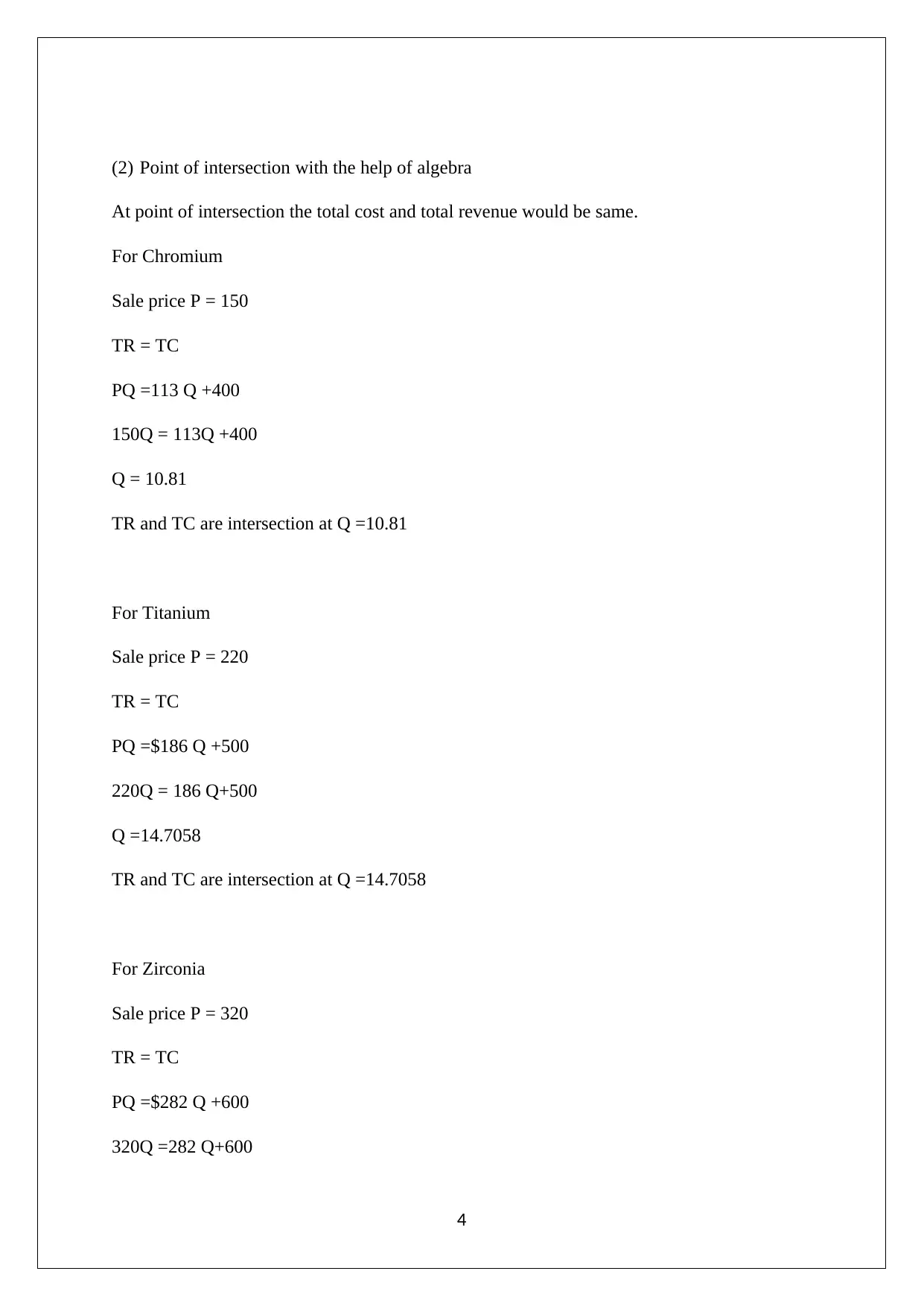
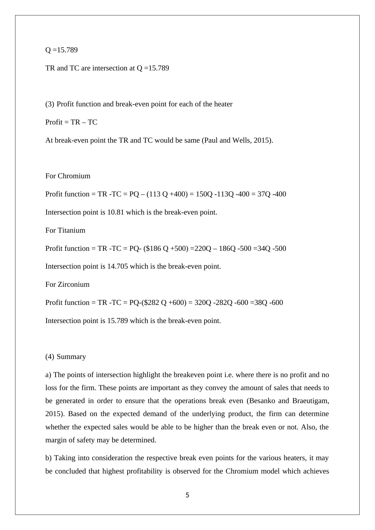
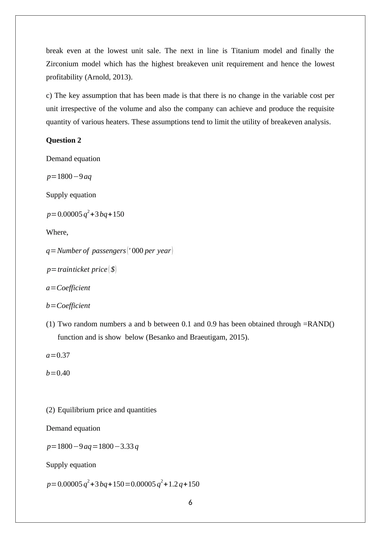
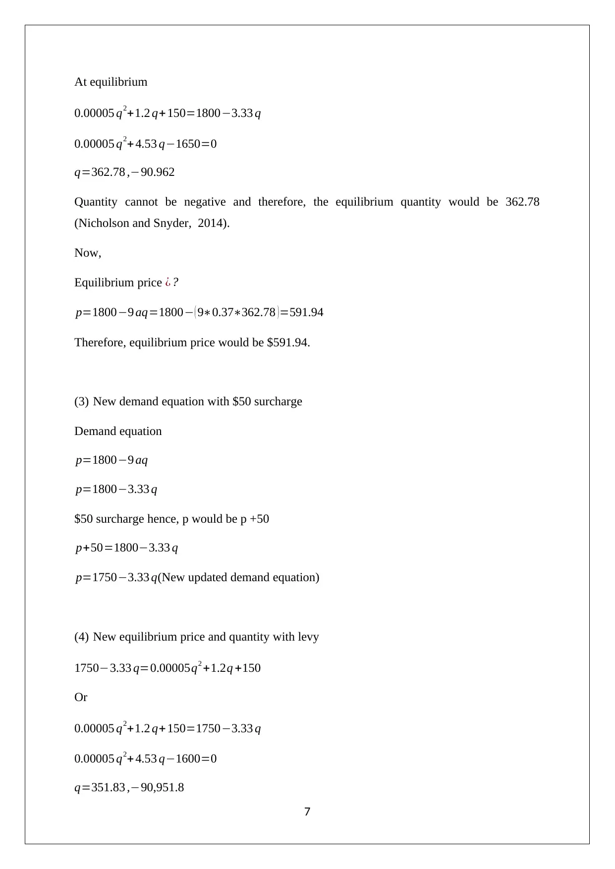
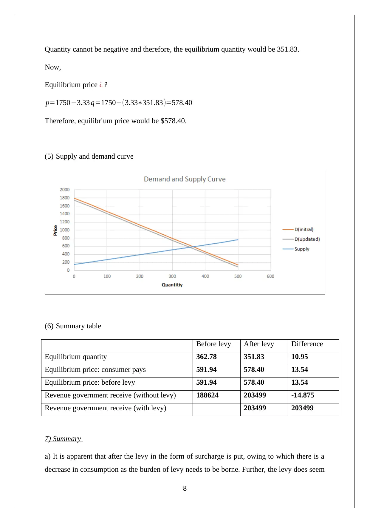
This project assignment for MAT10706, "Quantitative Methods with Economics," analyzes different casting methods, focusing on cost and revenue functions, break-even points, and profitability analysis. It calculates total costs, total revenue, and profit functions for three casting materials: Chromium, Titanium, and Zirconium, including Excel graphs for each. The assignment also examines supply and demand equations, determining equilibrium prices and quantities, and assesses the impact of a surcharge on demand. It uses algebraic methods to solve for intersection points and break-even points. The project concludes with a summary table comparing scenarios before and after a levy and discusses the implications of these analyses, considering assumptions and limitations. The assignment includes references to several economics textbooks.

QUANTITATIVE METHODS WITH ECONOMICS
STUDENT ID:
[Pick the date]

Question 1
The three different type of casting used by factory workers and their respective data and
information is shown below.
Chromium Titanium Zirconium
Cost of casting $75 $150 $240
Cost of gas fittings $38 $36 $42
Sale price $150 $220 $320
Fixed cost $400 $500 $600
Investigation
(1) Total cost and total revenue function along with excel graph
Total cost is a function of fixed cost and variable cost (Samuelson and Marks, 2013).
Variable cost
VC = Cost of casting + cost of gas fittings
For Chromium = 75 +38 = $113
For Titanium = 150 +36 =$186
For Zirconium = 240 +42 = $282
Total cost
TC = (Variable cost * Number of units) + Fixed Cost
Let number of units = Q
For Chromium = $113 Q +400
For Titanium =$186 Q +500
For Zirconium = $282 Q +600
Total revenue is a function of sale price and number of units (Nicholson and Snyder, 2014) .
TR = P Q
For Chromium
1

For Titanium
For Zirconium
Excel graph for TR and TC
2

1 2 3 4 5 6 7 8 9 10
$-
$1,000
$2,000
$3,000
$4,000
$5,000
$6,000
$7,000
$8,000
Chromium
TR & TC Curve
TR TC
1 2 3 4 5 6 7 8 9 10
$-
$2,000
$4,000
$6,000
$8,000
$10,000
$12,000
Titanium
TR & TC Curve
TR TC
1 2 3 4 5 6 7 8 9 10
$-
$2,000
$4,000
$6,000
$8,000
$10,000
$12,000
$14,000
$16,000
$18,000
Zirconium
TR & TC Curve
TR TC
3

(2) Point of intersection with the help of algebra
At point of intersection the total cost and total revenue would be same.
For Chromium
Sale price P = 150
TR = TC
PQ =113 Q +400
150Q = 113Q +400
Q = 10.81
TR and TC are intersection at Q =10.81
For Titanium
Sale price P = 220
TR = TC
PQ =$186 Q +500
220Q = 186 Q+500
Q =14.7058
TR and TC are intersection at Q =14.7058
For Zirconia
Sale price P = 320
TR = TC
PQ =$282 Q +600
320Q =282 Q+600
4

Q =15.789
TR and TC are intersection at Q =15.789
(3) Profit function and break-even point for each of the heater
Profit = TR – TC
At break-even point the TR and TC would be same (Paul and Wells, 2015).
For Chromium
Profit function = TR -TC = PQ – (113 Q +400) = 150Q -113Q -400 = 37Q -400
Intersection point is 10.81 which is the break-even point.
For Titanium
Profit function = TR -TC = PQ- ($186 Q +500) =220Q – 186Q -500 =34Q -500
Intersection point is 14.705 which is the break-even point.
For Zirconium
Profit function = TR -TC = PQ-($282 Q +600) = 320Q -282Q -600 =38Q -600
Intersection point is 15.789 which is the break-even point.
(4) Summary
a) The points of intersection highlight the breakeven point i.e. where there is no profit and no
loss for the firm. These points are important as they convey the amount of sales that needs to
be generated in order to ensure that the operations break even (Besanko and Braeutigam,
2015). Based on the expected demand of the underlying product, the firm can determine
whether the expected sales would be able to be higher than the break even or not. Also, the
margin of safety may be determined.
b) Taking into consideration the respective break even points for the various heaters, it may
be concluded that highest profitability is observed for the Chromium model which achieves
5

break even at the lowest unit sale. The next in line is Titanium model and finally the
Zirconium model which has the highest breakeven unit requirement and hence the lowest
profitability (Arnold, 2013).
c) The key assumption that has been made is that there is no change in the variable cost per
unit irrespective of the volume and also the company can achieve and produce the requisite
quantity of various heaters. These assumptions tend to limit the utility of breakeven analysis.
Question 2
Demand equation
p=1800−9 aq
Supply equation
p=0.00005 q2 +3 bq+150
Where,
q=Number of passengers (' 000 per year )
p=trainticket price ( $ )
a=Coefficient
b=Coefficient
(1) Two random numbers a and b between 0.1 and 0.9 has been obtained through =RAND()
function and is show below (Besanko and Braeutigam, 2015).
a=0.37
b=0.40
(2) Equilibrium price and quantities
Demand equation
p=1800−9 aq=1800−3.33 q
Supply equation
p=0.00005 q2 +3 bq+150=0.00005 q2 +1.2 q+150
6

At equilibrium
0.00005 q2+1.2 q+150=1800−3.33 q
0.00005 q2+4.53 q−1650=0
q=362.78 ,−90.962
Quantity cannot be negative and therefore, the equilibrium quantity would be 362.78
(Nicholson and Snyder, 2014).
Now,
Equilibrium price ¿ ?
p=1800−9 aq=1800− ( 9∗0.37∗362.78 )=591.94
Therefore, equilibrium price would be $591.94.
(3) New demand equation with $50 surcharge
Demand equation
p=1800−9 aq
p=1800−3.33 q
$50 surcharge hence, p would be p +50
p+50=1800−3.33 q
p=1750−3.33 q(New updated demand equation)
(4) New equilibrium price and quantity with levy
1750−3.33 q=0.00005q2 +1.2q +150
Or
0.00005 q2+1.2 q+150=1750−3.33 q
0.00005 q2+4.53 q−1600=0
q=351.83 ,−90,951.8
7

Quantity cannot be negative and therefore, the equilibrium quantity would be 351.83.
Now,
Equilibrium price ¿ ?
p=1750−3.33 q=1750−(3.33∗351.83)=578.40
Therefore, equilibrium price would be $578.40.
(5) Supply and demand curve
(6) Summary table
Before levy After levy Difference
Equilibrium quantity 362.78 351.83 10.95
Equilibrium price: consumer pays 591.94 578.40 13.54
Equilibrium price: before levy 591.94 578.40 13.54
Revenue government receive (without levy) 188624 203499 -14.875
Revenue government receive (with levy) 203499 203499
7) Summary
a) It is apparent that after the levy in the form of surcharge is put, owing to which there is a
decrease in consumption as the burden of levy needs to be borne. Further, the levy does seem
8

to be productive from the perspective of the government as it has not impacted the
consumption of services but has led to higher revenue generation for the government. This is
on expected lines as for train service the demand would be expected to be inelastic (Pindyck
and Rubinfeld, 2014).
b) Considering the positive impact of the levy on the government revenues, it makes sense
that levy ought to be introduced. This would provide much needed support for the financial
situation of the government and help it to maintain the quality of the services in the wake of
the higher operating costs (Mankiw,2014).
c) The tacit assumption is that the supply can adjust without any changes in cost to the
variations in demand in a short period of time. Typically this is not the case owing to which
the utility of the analysis conducted may be limited.
Referencing
Arnold, A.R. (2013). Microeconomics (9th ed.). Sydney: Cengage Learning.
9

Besanko, D. and Braeutigam, R. (2015). Microeconomics (4th ed.). New York: John Wiley &
Sons.
Mankiw, G. (2014) Microeconomics (6th ed.). London: Worth Publishers.
Nicholson, W. and Snyder, C. (2014). Fundamentals of Economics (11th ed.). New York:
Cengage Learning.
Paul, K. and Wells, R. (2015). Microeconomics (2nd ed.). London: Worth Publishers.
Pindyck, R. and Rubinfeld, D. (2014). Microeconomics (5th ed.). London: Prentice-Hall
Publications.
Samuelson, W. and Marks, S. (2013). Managerial Economics (4th ed.). New York: Wiley
Publications.
10