MAT540 Week 10 Homework: Chapter 13 Queuing Analysis Problems

This document presents a comprehensive solution to a queuing analysis homework assignment, addressing several problems related to waiting line systems. The assignment explores various scenarios, including single-server and multi-server queuing models, and analyzes key performance indicators such as average queue length, waiting time, and system utilization. The solutions demonstrate the application of queuing theory to optimize service operations, evaluate the impact of adding servers or resources, and make informed decisions regarding cost-benefit trade-offs. The document includes calculations, interpretations, and recommendations based on the analysis of different queuing scenarios, providing a practical understanding of queuing concepts and their application in real-world business contexts, specifically within the realm of management science. The assignment covers topics like calculating the impact of increased arrival rates, evaluating the cost-effectiveness of adding service windows, and determining the optimal number of servers to minimize waiting times and maximize revenue. Moreover, the document incorporates references to relevant academic sources to support the analysis and conclusions.

Running head: QUANTUM MATHEMATICS 1
Quantum Mathematics
Student Name
Institution

QUANTUM MATHEMATICS 2
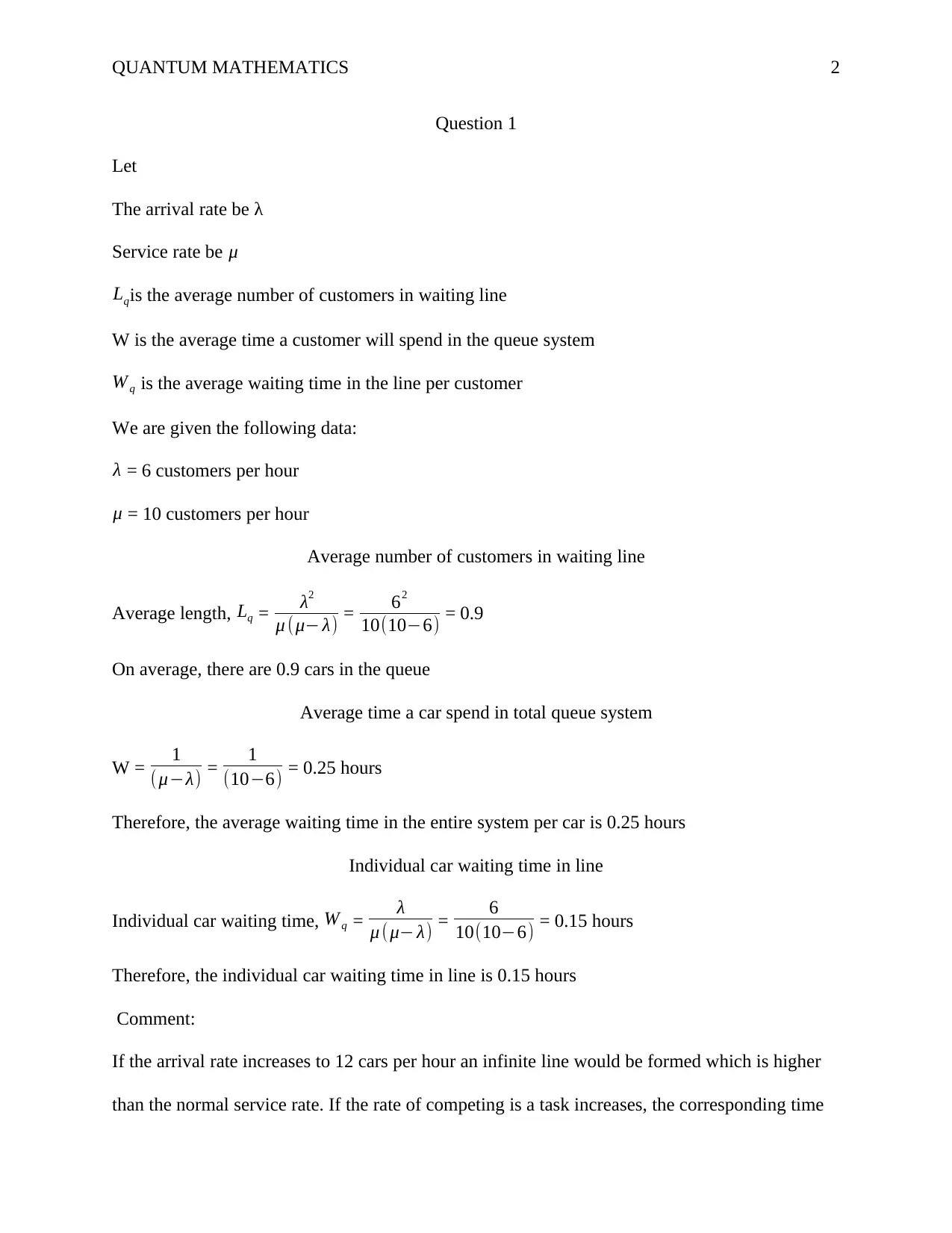
Question 1
Let
The arrival rate be λ
Service rate be μ
Lqis the average number of customers in waiting line
W is the average time a customer will spend in the queue system
W q is the average waiting time in the line per customer
We are given the following data:
λ = 6 customers per hour
μ = 10 customers per hour
Average number of customers in waiting line
Average length, Lq = λ2
μ (μ− λ) = 62
10(10−6) = 0.9
On average, there are 0.9 cars in the queue
Average time a car spend in total queue system
W = 1
( μ−λ) = 1
(10−6) = 0.25 hours
Therefore, the average waiting time in the entire system per car is 0.25 hours
Individual car waiting time in line
Individual car waiting time, Wq = λ
μ (μ− λ) = 6
10(10−6) = 0.15 hours
Therefore, the individual car waiting time in line is 0.15 hours
Comment:
If the arrival rate increases to 12 cars per hour an infinite line would be formed which is higher
than the normal service rate. If the rate of competing is a task increases, the corresponding time

QUANTUM MATHEMATICS 3
for completing the task decreases significantly (Ocampo, Paycha & Reyes, 2001; Wrede, Spiegel
& Arangno, 2002).
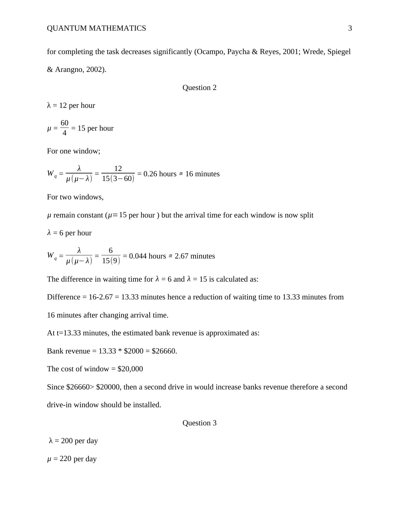
Question 2
λ = 12 per hour
μ = 60
4 = 15 per hour
For one window;
W q = λ
μ (μ− λ) = 12
15(3−60) = 0.26 hours ≅ 16 minutes
For two windows,
μ remain constant (μ=15 per hour ) but the arrival time for each window is now split
λ = 6 per hour
W q = λ
μ (μ− λ) = 6
15(9) = 0.044 hours ≅ 2.67 minutes
The difference in waiting time for λ = 6 and λ = 15 is calculated as:
Difference = 16-2.67 = 13.33 minutes hence a reduction of waiting time to 13.33 minutes from
16 minutes after changing arrival time.
At t=13.33 minutes, the estimated bank revenue is approximated as:
Bank revenue = 13.33 * $2000 = $26660.
The cost of window = $20,000
Since $26660> $20000, then a second drive in would increase banks revenue therefore a second
drive-in window should be installed.
Question 3
λ = 200 per day
μ = 220 per day

QUANTUM MATHEMATICS 4
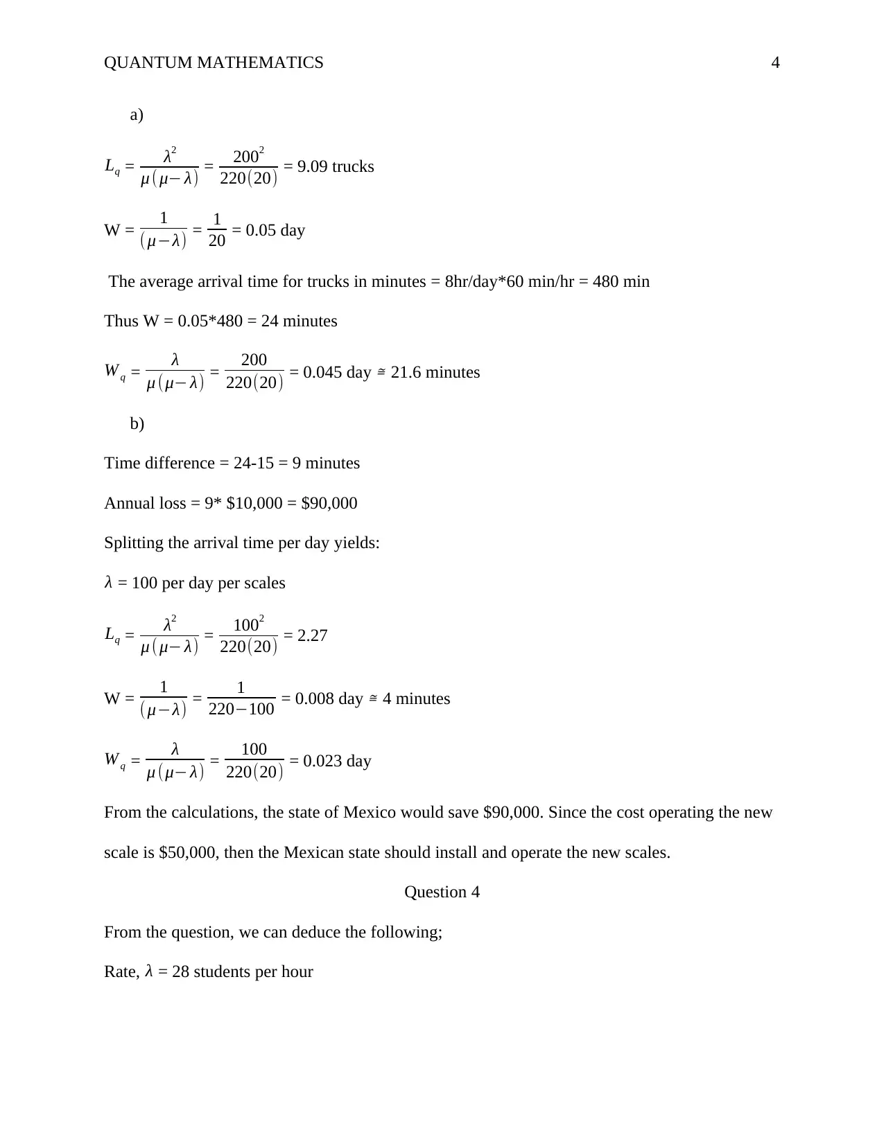
a)
Lq = λ2
μ ( μ− λ) = 2002
220(20) = 9.09 trucks
W = 1
( μ−λ) = 1
20 = 0.05 day
The average arrival time for trucks in minutes = 8hr/day*60 min/hr = 480 min
Thus W = 0.05*480 = 24 minutes
W q = λ
μ (μ− λ) = 200
220(20) = 0.045 day ≅ 21.6 minutes
b)
Time difference = 24-15 = 9 minutes
Annual loss = 9* $10,000 = $90,000
Splitting the arrival time per day yields:
λ = 100 per day per scales
Lq = λ2
μ ( μ− λ) = 1002
220(20) = 2.27
W = 1
( μ−λ) = 1
220−100 = 0.008 day ≅ 4 minutes
W q = λ
μ (μ− λ) = 100
220(20) = 0.023 day
From the calculations, the state of Mexico would save $90,000. Since the cost operating the new
scale is $50,000, then the Mexican state should install and operate the new scales.
Question 4
From the question, we can deduce the following;
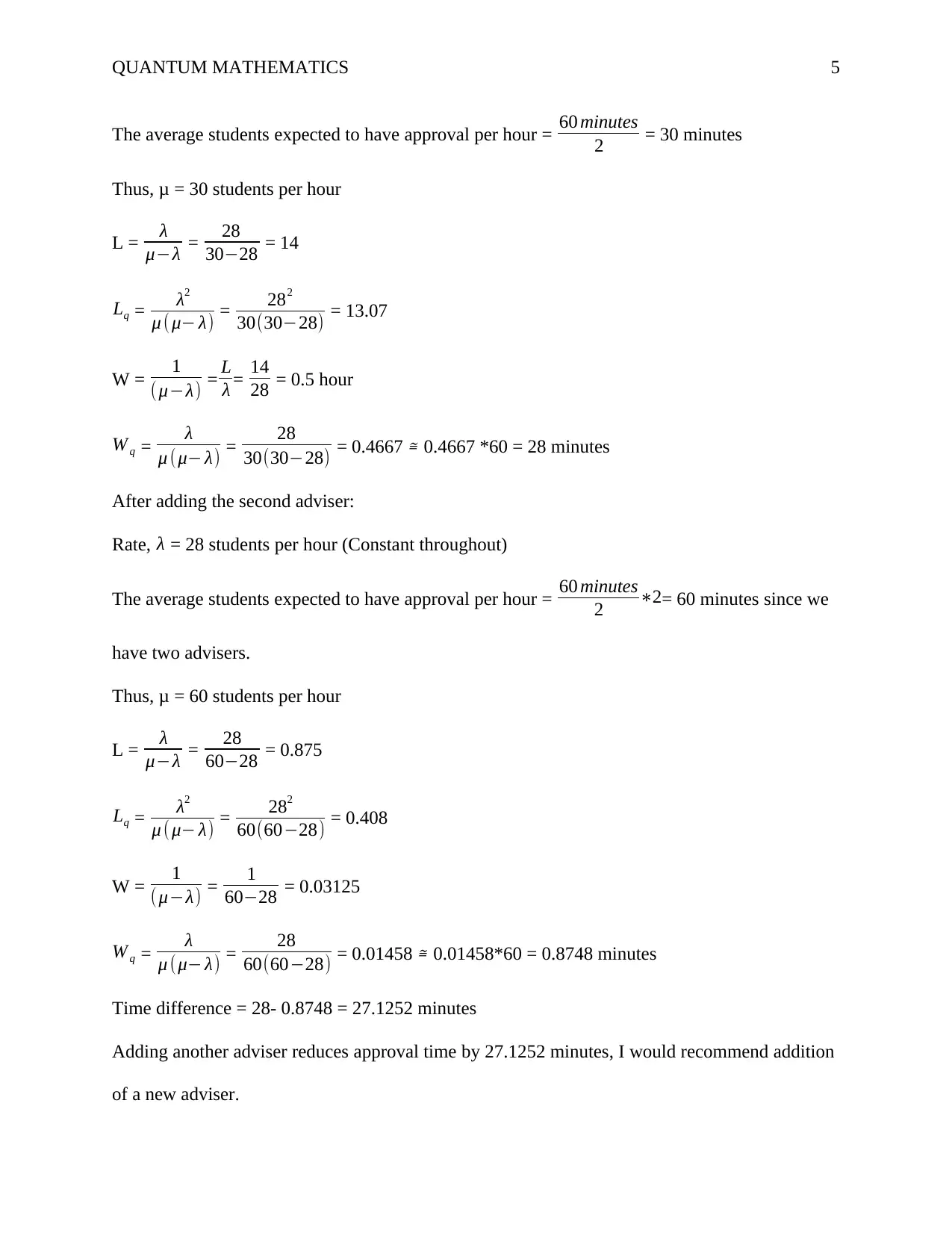
Rate, λ = 28 students per hour

QUANTUM MATHEMATICS 5
The average students expected to have approval per hour = 60 minutes
2 = 30 minutes
Thus, μ = 30 students per hour
L = λ
μ−λ = 28
30−28 = 14
Lq = λ2
μ ( μ− λ) = 282
30(30−28) = 13.07
W = 1
( μ−λ) = L
λ = 14
28 = 0.5 hour
W q = λ
μ (μ− λ) = 28
30(30−28) = 0.4667 ≅ 0.4667 *60 = 28 minutes
After adding the second adviser:
Rate, λ = 28 students per hour (Constant throughout)
The average students expected to have approval per hour = 60 minutes
2 ∗2= 60 minutes since we
have two advisers.
Thus, μ = 60 students per hour
L = λ
μ−λ = 28
60−28 = 0.875
Lq = λ2
μ ( μ− λ) = 282
60(60−28) = 0.408
W = 1
( μ−λ) = 1
60−28 = 0.03125
W q = λ
μ (μ− λ) = 28
60(60−28) = 0.01458 ≅ 0.01458*60 = 0.8748 minutes
Time difference = 28- 0.8748 = 27.1252 minutes
Adding another adviser reduces approval time by 27.1252 minutes, I would recommend addition
of a new adviser.

QUANTUM MATHEMATICS 6
Question 5
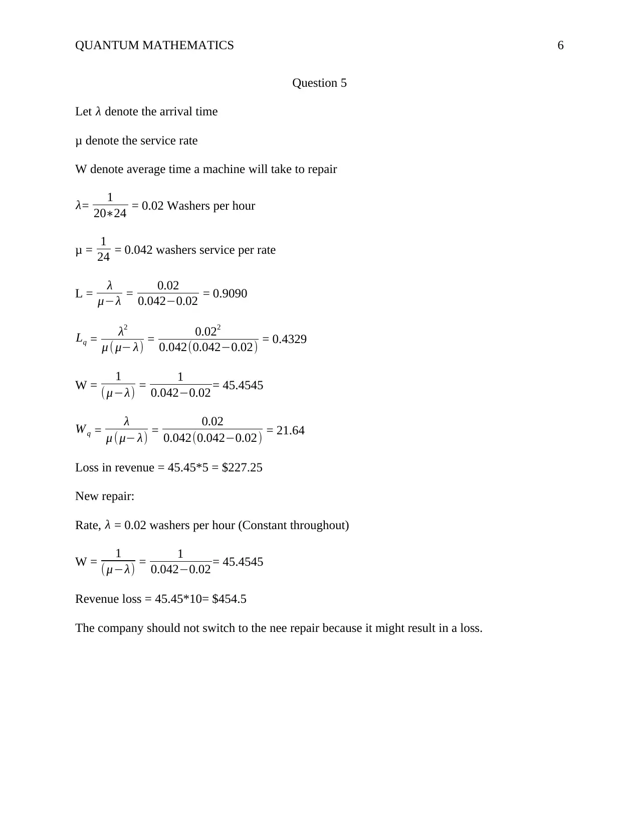
Let λ denote the arrival time
μ denote the service rate
W denote average time a machine will take to repair
λ= 1
20∗24 = 0.02 Washers per hour
μ = 1
24 = 0.042 washers service per rate
L = λ
μ−λ = 0.02
0.042−0.02 = 0.9090
Lq = λ2
μ ( μ− λ) = 0.022
0.042(0.042−0.02) = 0.4329
W = 1
( μ−λ) = 1
0.042−0.02 = 45.4545
W q = λ
μ (μ− λ) = 0.02
0.042(0.042−0.02) = 21.64
Loss in revenue = 45.45*5 = $227.25
New repair:
Rate, λ = 0.02 washers per hour (Constant throughout)
W = 1
( μ−λ) = 1
0.042−0.02 = 45.4545
Revenue loss = 45.45*10= $454.5
The company should not switch to the nee repair because it might result in a loss.

QUANTUM MATHEMATICS 7
References
Ocampo, H., Paycha, S., & Reyes, A. (2001). Geometric methods for quantum field theory.
Singapore: World Scientific.
Wrede, R., Spiegel, M., & Arangno, D. (2002). Schaum's outline of theory and problems of
advanced calculus. New York: McGraw Hill.