MATH1111 Maths Assignment: Transformations, Graphs & Analysis 2019

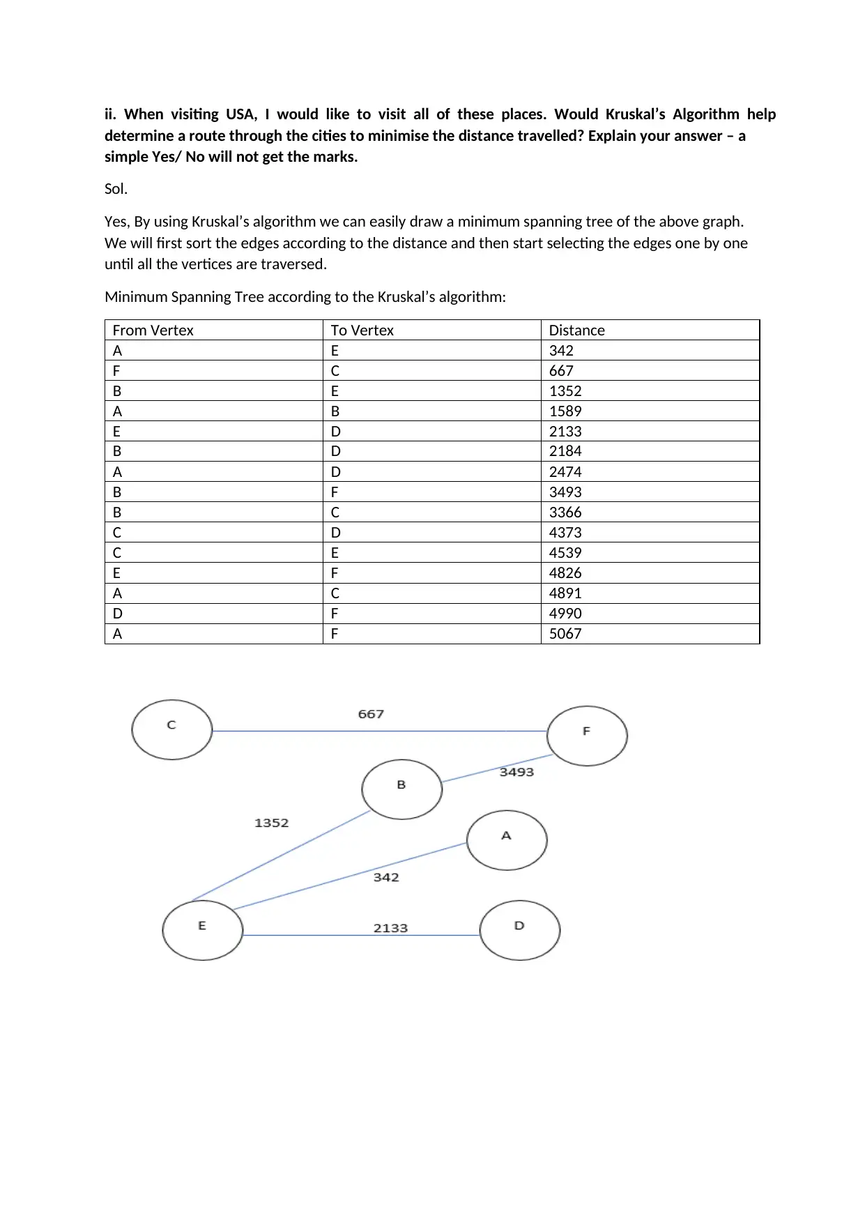
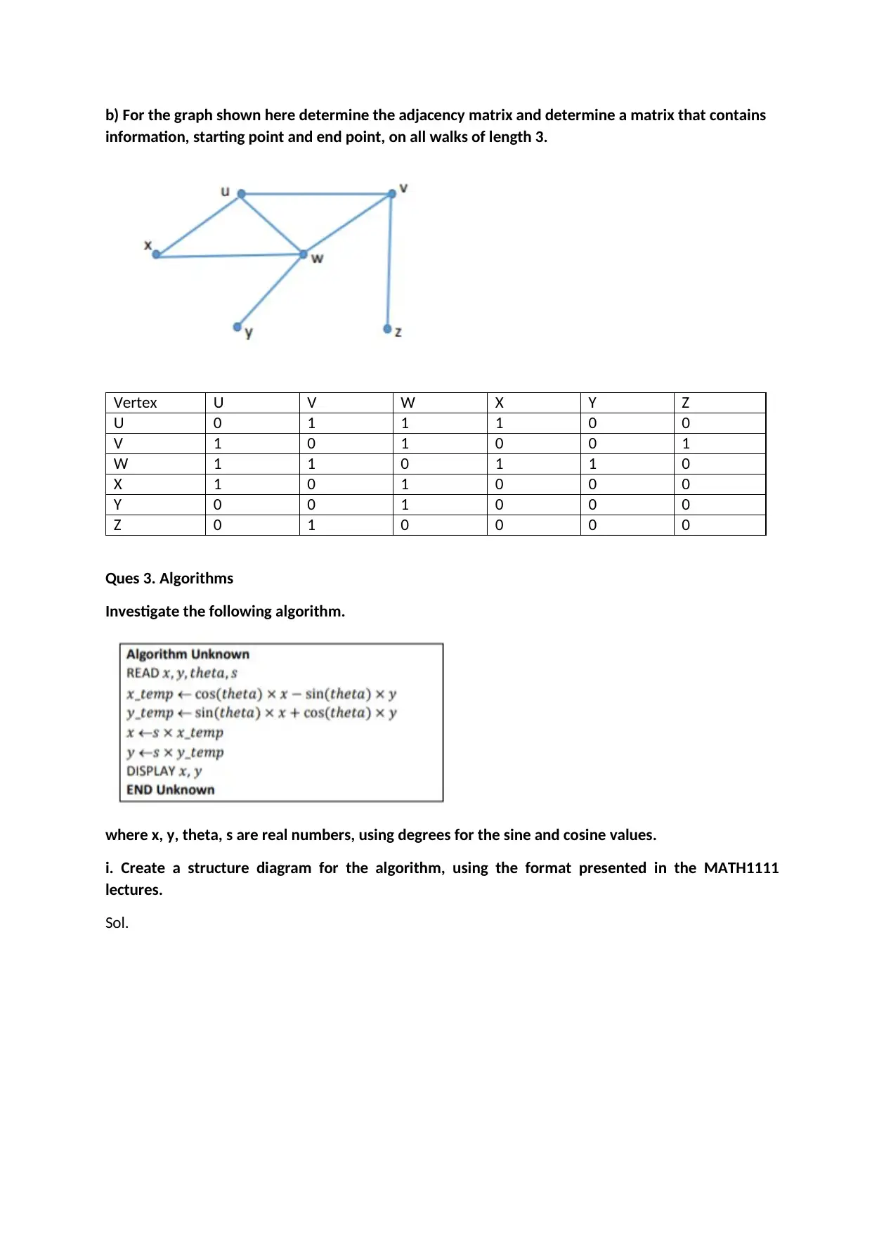
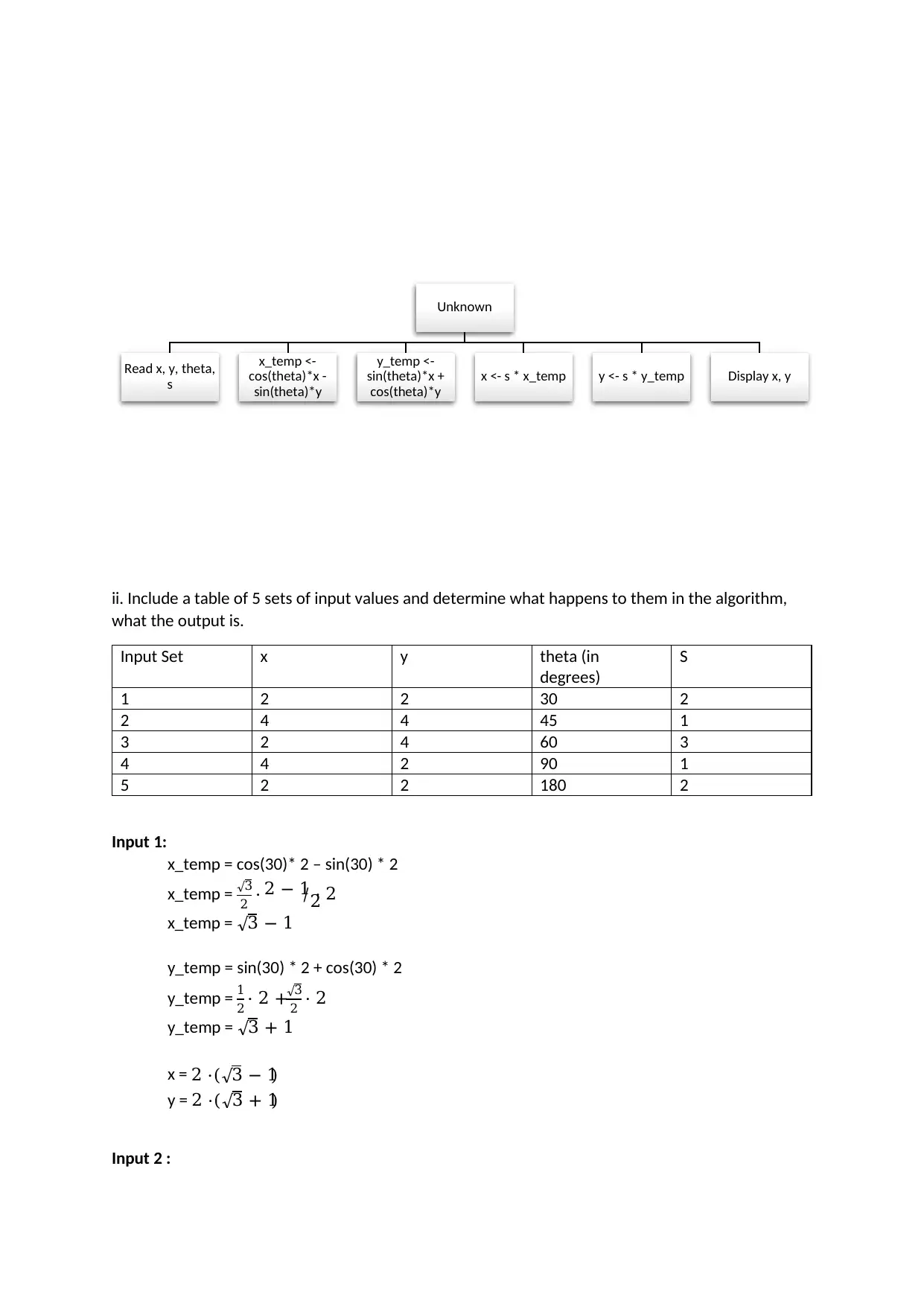
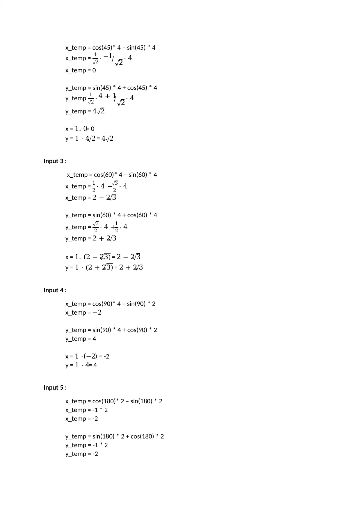
This assignment solution covers several key mathematical concepts. It begins with quadrilateral transformations, including rotations and scaling, visualized on a graph. Next, it explores graph theory, applying Kruskal's algorithm to find the minimum distance between cities and analyzing adjacency matrices. The assignment then delves into algorithm analysis, including structure diagrams and input-output analysis. Calculus is addressed through differentiation and integration problems. Finally, the assignment covers data visualization, presenting temperature data in a graph and calculating descriptive statistics. Desklib offers a wealth of similar solved assignments and study resources for students.

MATHS ASSIGNMENT
MARCH 19, 2019

A=1
B=1
C=5
D=6
E=8
F=9
Ques 1. Write down the quadrilateral Q =
i. Draw its position on a graph.
On substituting values, we get the coordinates as W (1,1), X (10,1), Y (10,10) & Z (1,9)
ii. Write down a matrix R that will rotate Q 90 degrees anti clockwise around the origin.
R =
( −1 −1 −10 −9
1 10 10 1 )
iii. Write down a matrix T that will rotate Q 90 degrees anticlockwise around the origin and increase
the size of Q by a factor 2.
T =
( −2 −2 −20 −18
2 20 20 2 )
0
1
2
3
4
5
6
7
8
9
10
11
0 1 2 3 4 5 6 7 8 9 10 11
W (1,1) X (10,1)
Y (10,10)
Z (1,9)

iv. Use the transformations on Q and draw the transformed quadrilaterals RQ and TQ on the graph.
Make sure to clearly label the quadrilaterals.
R =
T =
v. Calculate the matrices R4 and T4 and explain your answers.
0
1
2
3
4
5
6
7
8
9
10
11
-11 -10 -9 -8 -7 -6 -5 -4 -3 -2 -1 0
0
1
2
3
4
5
6
7
8
9
10
11
12
13
14
15
16
17
18
19
20
21
-21 -20 -19 -18 -17 -16 -15 -14 -13 -12 -11 -10 -9 -8 -7 -6 -5 -4 -3 -2 -1 0
W’ (-1,1)
X’ (-1,10)Y’ (-10,10)
Z’ (-9,1)
W’’ (-2,2)
X’’ (-2,20)Y’’ (-20,20)
Z’’ (-18,2)

Sol.
These can not be calculated as the matrices R and T are not square matrices.
Ques 2. Graph Theory
a) The following distance table shows the distance in kilometres between some cities in the USA.
Distance
(km)
Boston Chicago Los Angeles Miami New York San
Francisco
Boston 1589 4891 2474 342 5067
Chicago 3366 2184 1352 3493
Los Angeles 4373 4539 667
Miami 2133 4990
New York 4826
i. Draw this information as a graph.
Solution:
Vertices:
City Vertex
Boston A
Chicago B
Los Angeles C
Miami D
New York E
San Francisco F

ii. When visiting USA, I would like to visit all of these places. Would Kruskal’s Algorithm help
determine a route through the cities to minimise the distance travelled? Explain your answer – a
simple Yes/ No will not get the marks.
Sol.
Yes, By using Kruskal’s algorithm we can easily draw a minimum spanning tree of the above graph.
We will first sort the edges according to the distance and then start selecting the edges one by one
until all the vertices are traversed.
Minimum Spanning Tree according to the Kruskal’s algorithm:
From Vertex To Vertex Distance
A E 342
F C 667
B E 1352
A B 1589
E D 2133
B D 2184
A D 2474
B F 3493
B C 3366
C D 4373
C E 4539
E F 4826
A C 4891
D F 4990
A F 5067

b) For the graph shown here determine the adjacency matrix and determine a matrix that contains
information, starting point and end point, on all walks of length 3.
Vertex U V W X Y Z
U 0 1 1 1 0 0
V 1 0 1 0 0 1
W 1 1 0 1 1 0
X 1 0 1 0 0 0
Y 0 0 1 0 0 0
Z 0 1 0 0 0 0
Ques 3. Algorithms
Investigate the following algorithm.
where x, y, theta, s are real numbers, using degrees for the sine and cosine values.
i. Create a structure diagram for the algorithm, using the format presented in the MATH1111
lectures.
Sol.

ii. Include a table of 5 sets of input values and determine what happens to them in the algorithm,
what the output is.
Input Set x y theta (in
degrees)
S
1 2 2 30 2
2 4 4 45 1
3 2 4 60 3
4 4 2 90 1
5 2 2 180 2
Input 1:
x_temp = cos(30)* 2 – sin(30) * 2
x_temp = √3
2 ⋅ 2 − 12⁄ ⋅ 2
x_temp = √3 − 1
y_temp = sin(30) * 2 + cos(30) * 2
y_temp = 1
2 ⋅ 2 +√3
2 ⋅ 2
y_temp = √3 + 1
x = 2 ⋅(√3 − 1)
y = 2 ⋅(√3 + 1)
Input 2 :
Unknown
Read x, y, theta,
s
x_temp <-
cos(theta)*x -
sin(theta)*y
y_temp <-
sin(theta)*x +
cos(theta)*y
x <- s * x_temp y <- s * y_temp Display x, y

x_temp = cos(45)* 4 – sin(45) * 4
x_temp = 1
√2 ⋅ −1
√2
⁄ ⋅ 4
x_temp = 0
y_temp = sin(45) * 4 + cos(45) * 4
y_temp 1
√2 ⋅ 4 + 1
√2
⁄ ⋅ 4
y_temp = 4√2
x = 1. 0= 0
y = 1 ⋅ 4√2 = 4√2
Input 3 :
x_temp = cos(60)* 4 – sin(60) * 4
x_temp = 1
2 ⋅ 4 −√3
2 ⋅ 4
x_temp = 2 − 2√3
y_temp = sin(60) * 4 + cos(60) * 4
y_temp = √3
2 ⋅ 4 +1
2 ⋅ 4
y_temp = 2 + 2√3
x = 1. (2 − 2√3) = 2 − 2√3
y = 1 ⋅ (2 + 2√3) = 2 + 2√3
Input 4 :
x_temp = cos(90)* 4 – sin(90) * 2
x_temp = −2
y_temp = sin(90) * 4 + cos(90) * 2
y_temp = 4
x = 1 ⋅(−2) = -2
y = 1 ⋅ 4= 4
Input 5 :
x_temp = cos(180)* 2 – sin(180) * 2
x_temp = -1 * 2
x_temp = -2
y_temp = sin(180) * 2 + cos(180) * 2
y_temp = -1 * 2
y_temp = -2

x = 2. (−2)= -4
y = 2 ⋅ (−2)= −4
iii. Explain what the algorithm does and what the output values are.
Sol.
The algorithm computes the values of two variables x and y by using some trigonometric functions
and finally print the values.
The outputs for the above set of input values are as follows:
Input X Y
1 2 ⋅(√3 − 1) 2 ⋅(√3 + 1)
2 0 4√2
3 2 − 2√3 2 + 2√3
4 -2 4
5 -4 -4
iv. Modify the algorithm to allow x, y to be arrays. What would be the purpose of the algorithm be
then?
If x and y are modified to be arrays then, the steps would change, we will only change the input
values and for each input, the outputs x and y will be automatically stored in the array.
Ques 4. Differentiation and Integration
a) Find dy/dx for the function y = Cx3 -3x +Dsin(2x) -4
Sol.
Substituting the values of variables:
y = 5x3 – 3x + 6sin2x -4
𝑑𝑦
𝑑𝑥= 15𝑥2 − 3 + 6.2𝑐𝑜𝑠2𝑥
𝑑𝑦
𝑑𝑥= 15𝑥2 − 3 + 12𝑐𝑜𝑠2𝑥
b) Use the product rule to find dy/dx for y= xF cos(Dx).
Sol. Substituting the values of variables:
𝑦 = 9𝑥. 𝑐𝑜𝑠6𝑥
𝑑𝑦
𝑑𝑥= 9𝑐𝑜𝑠6𝑥 + 9𝑥. (−6𝑠𝑖𝑛6𝑥)
𝑑𝑦
𝑑𝑥= 9𝑐𝑜𝑠6𝑥 − 54𝑥𝑠𝑖𝑛6𝑥
c) Find the values of the following integrals.

i.
Sol. Substituting the values of the variables:
𝐼 = ∫ 6𝑥2 + 𝑒𝑥 + 1 𝑑𝑥
2
1
𝐼 = [2𝑥3 + 𝑒𝑥 + 𝑥 ]1
2
= (24 + 𝑒2 + 2) − (2 + 𝑒 + 1)
= 15 + 𝑒2 − 𝑒
ii.
Sol. Substituting the values of variables:
𝐼 = ∫ 𝑐𝑜𝑠𝑥 − 𝑥9
= 𝑠𝑖𝑛𝑥 −
𝑥10
10 + 𝑐
d) Given f(x)= Cx -x2
f(x) = 5x -x2
i. Plot the function f(x) over the interval [0,C].
ii. Differentiate f(x) and determine the value of df/dx when x=0. What does df/dx represent? Show
on your graph from d)i. option.
𝑑𝑦
𝑑𝑥= 5 − 2𝑥
0
1
2
3
4
5
6
7
0 1 2 3 4 5 6 7
f(x)

𝑑𝑦
𝑑𝑥|𝑥=0 = 5 − 2(0)
= 5
This represents the slope of the function f(x).
Ques 5. Data Visualisation and Presentation
The table shows below the temperature recorded in Basel from 1989 – 2019. Specifically, the
temperature has been recorded at midnight 1st March 2 metres above ground every year.
Year Temperature (in degree centigrade)
1989 6.33
1990 6.44
1991 10.24
1992 15.77
1993 2.64
1994 11.92
1995 11.88
1996 5.86
1997 15.77
1998 7.86
1999 8.14
2000 8.11
2001 5.28
2002 12.25
2003 12.53
2004 1.56
2005 -4.80
2006 -0.32
2007 9.61
2008 11.50
2009 11.35
2010 8.10
2011 5.55
2012 12.02
2013 3.89
2014 7.56
2015 10.49
2016 4.62
2017 7.14
2018 -0.31
2019 9.14
i. Use an appropriate graph in Excel to display the data, include a printed version in the assignment
submission.

ii. Obtain descriptive statistics values for the data to include – Minimum, Maximum, Mean, Median,
Mode, range, Sample standard deviation, sample variance, population variance. Include working
and/or excel sheets.
Sample Excel screenshot
Results:
6.336.44
10.24
15.77
2.64
11.9211.88
5.86
15.77
7.868.148.11
5.28
12.2512.53
1.56
-4.8
-0.32
9.61
11.511.35
8.1
5.55
12.02
3.89
7.56
10.49
4.62
7.14
-0.31
9.14
-10
-5
0
5
10
15
20
1989
1990
1991
1992
1993
1994
1995
1996
1997
1998
1999
2000
2001
2002
2003
2004
2005
2006
2007
2008
2009
2010
2011
2012
2013
2014
2015
2016
2017
2018
2019
Temperature (in degrees centigrade)
Year