MATH2001 Assignment 4 Solution: Vector Fields and Green's Theorem
VerifiedAdded on 2023/03/17
|6
|1302
|62
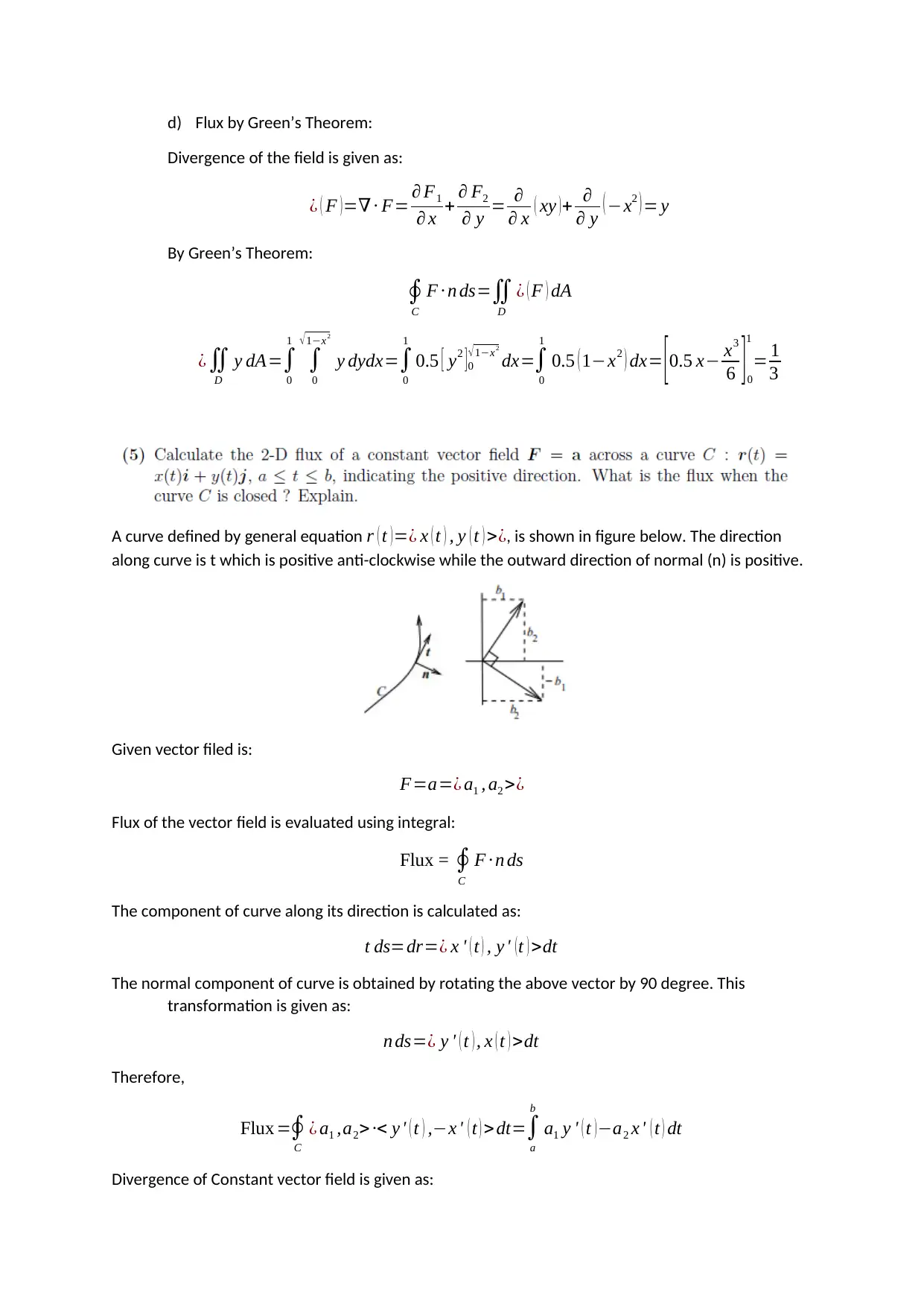
Homework Assignment
AI Summary
This document provides a comprehensive solution to MATH2001 Assignment 4, focusing on vector calculus concepts. The solution begins by evaluating line integrals along different paths for a given vector field, including a parabola and a straight line, and determining if the field is conservative. It then proceeds to evaluate a line integral along a helical path for a second vector field and finds the corresponding potential function. The assignment also covers the application of Green's Theorem, calculating both line integrals and double integrals to find the flux of a vector field over a given path, including the use of parametric equations to define the path. The solution demonstrates the calculation of the flux over sub-paths and utilizes Green's Theorem to verify the results, providing a detailed analysis of vector fields, line integrals, and flux calculations.
1 out of 6
Related Documents


Your All-in-One AI-Powered Toolkit for Academic Success.
+13062052269
info@desklib.com
Available 24*7 on WhatsApp / Email
![[object Object]](/_next/static/media/star-bottom.7253800d.svg)
Copyright © 2020–2026 A2Z Services. All Rights Reserved. Developed and managed by ZUCOL.