MATH 240 Project: Applying MATLAB for Advanced Matrix Analysis

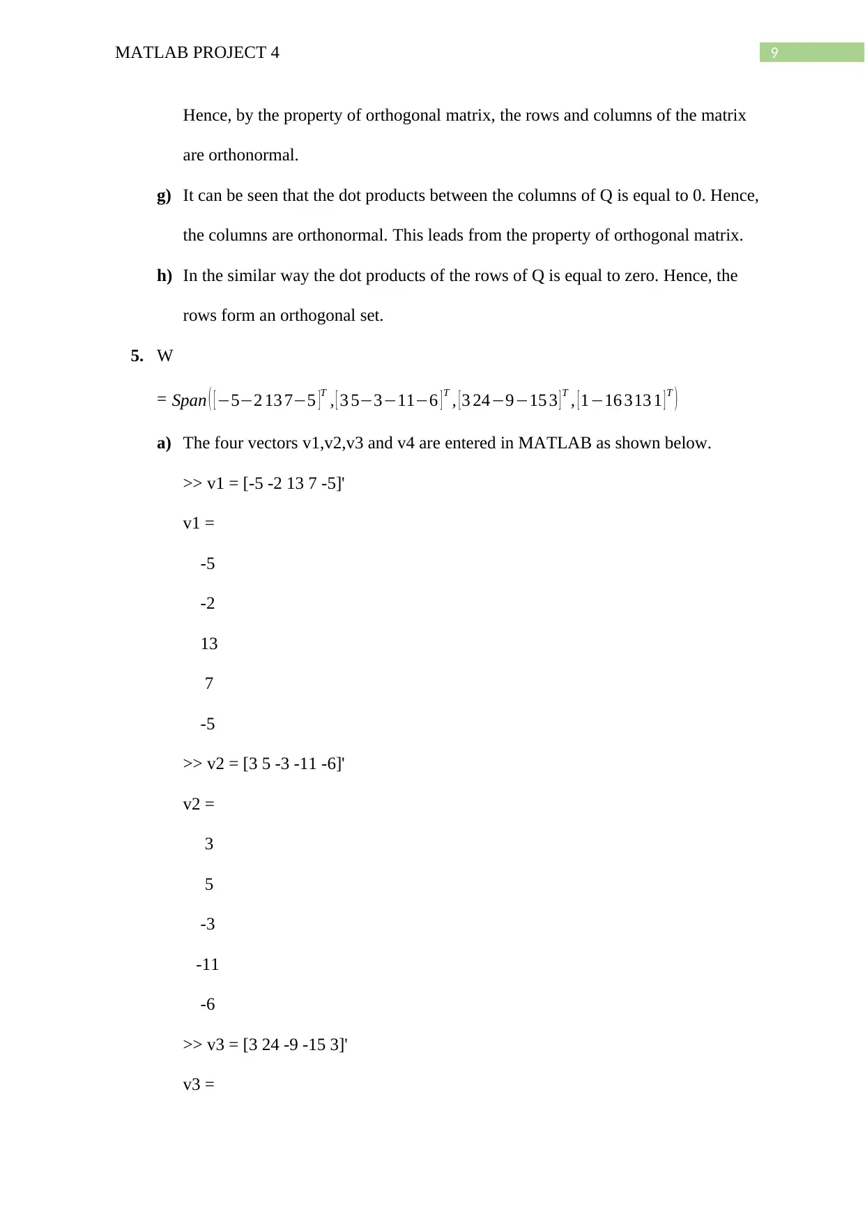
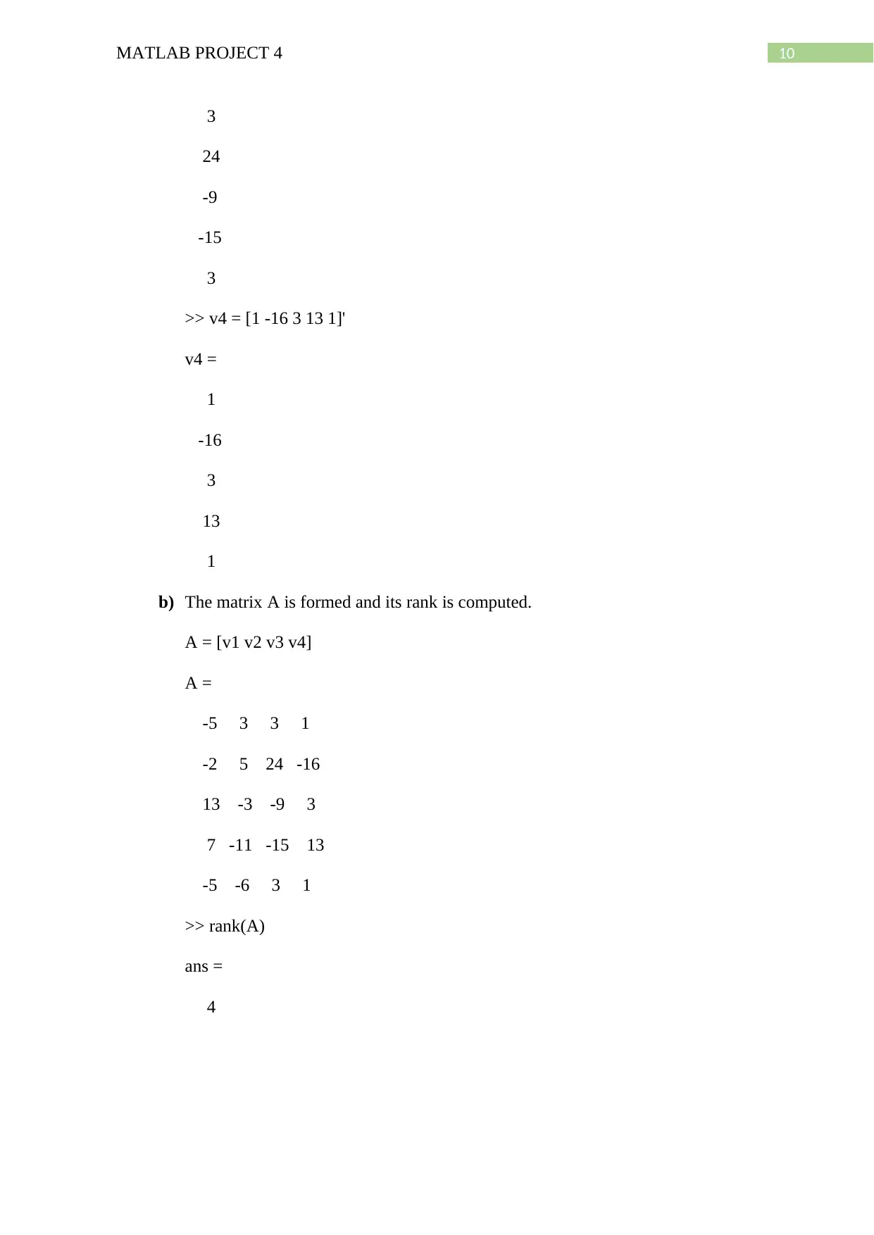
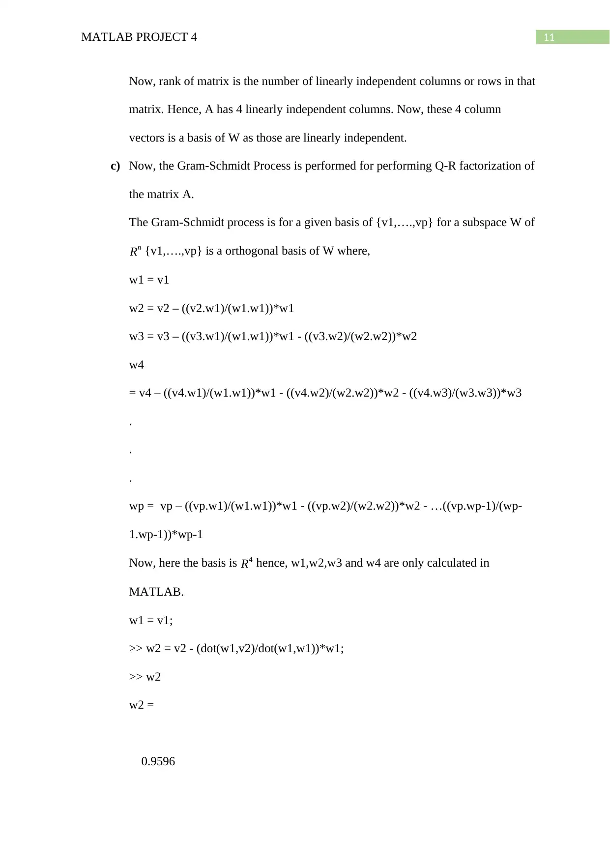
This assignment focuses on utilizing MATLAB to explore various concepts in linear algebra, particularly matrix diagonalization. It begins by demonstrating how to use MATLAB to find eigenvalues and eigenvectors of given matrices. The assignment then verifies the diagonalization process and uses the results to compute powers of matrices. The Gram-Schmidt process is applied to find orthogonal and orthonormal bases for a given subspace. Additionally, the assignment investigates the properties of orthogonal matrices and their relationship to orthonormal sets. The document showcases detailed MATLAB commands and outputs, providing a step-by-step guide to solving linear algebra problems using computational tools. This resource is available on Desklib, which offers a range of study tools, including past papers and solved assignments, to support student learning.

Running head: MATLAB PROJECT 4
MATH 240
MATLAB PROJECT 4
Name of the Student
Name of the University
Author Note

1MATLAB PROJECT 4
0. The command clock is entered in MATLAB which displays the current year, month,
date and time in the following format.
[year month day hour minute seconds]
MATLAB command and output:
clock
ans =
2018 11 26 12 40 32.391
Hence, the current date and time is 26th November 2018, 12 PM 40 minutes and
32.391 secs.
1. The matrix A = [ 345 −654 −928
84 −158 −228
66 −126 −176 ]
The diagonalization of the matrix A is performed by the following method.
A=P∗D∗P−1
Where, D is the diagonal matrix and P is the eigenvector matrix which is invertible.
Matrix diagonalization is very much useful in computation of An where n is any
positive integer.
a) A =[345 -654 -928;84 -158 -228;66 -126 -176]
A =
345 -654 -928
84 -158 -228
66 -126 -176
[P,D] = eig(A)
P =
0.95702 -0.94561 0.9577
0.20508 -0.29096 0.15962

2MATLAB PROJECT 4
0.20508 -0.14548 0.23943
D =
6 0 0
0 1 0
0 0 4
b) Now, in MATLAB diagonalization is verified.
P*D*P^(-1)
ans =
345 -654 -928
84 -158 -228
66 -126 -176
Hence, as the matrix is equal to A, it can be said that diagonalization is performed
correctly by MATLAB.
c) Now, by using the previous results the eigenvectors and their corresponding Eigen
values are given below.
Eigen value = 6, Eigen vector = [0.95702
0.20508
0.20508 ]
Eigen value = 1, Eigen vector = [−0.94561
−0.29096
−0.14548 ]
Eigen value = 4, Eigen vector = [ 0.9577
0.15962
0.23943 ]
2. The given matrix A = [−65 −39 −15
100 60 23
22 13 6 ]
a) In MATLAB values of An for n = 2,3,4,5,6,7,8 are obtained as follows.
>> A^2

3MATLAB PROJECT 4
ans =
-5 0 -12
6 -1 18
2 0 5
>> A^3
ans =
61 39 3
-94 -60 -5
-20 -13 0
>> A^4
ans =
1 0 0
0 1 0
0 0 1
>> A^5
ans =
-65 -39 -15
100 60 23
22 13 6
>> A^6
ans =
-5 0 -12
6 -1 18
2 0 5
>> A^7

4MATLAB PROJECT 4
ans =
61 39 3
-94 -60 -5
-20 -13 0
>> A^8
ans =
1 0 0
0 1 0
0 0 1
Hence, a pattern is observed which repeats for every n=4 increments. The matrixes
are same for n=1,2,3,4 and n=5,6,7 and 8.
b) Now, the matrix diagonalization is performed like the previous way.
[P,D] = eig(A)
P =
-0.53609 + 0.0089348i -0.53609 - 0.0089348i -0.53452 + 0i
0.82498 + 0i 0.82498 + 0i 0.80178 + 0i
0.1787 - 0.0029783i 0.1787 + 0.0029783i 0.26726 + 0i
D =
-8.8523e-15 + 1i 0 + 0i 0 + 0i
0 + 0i -8.8523e-15 - 1i 0 + 0i
0 + 0i 0 + 0i 1 + 0i
Hence, it is seen that there are two Eigen values that are complex numbers and
one is real number. All the Eigen vectors corresponding to their Eigen values are
complex vectors.
c) Now, An =P∗Dn∗P−1, where n is any positive integer.

5MATLAB PROJECT 4
So, the powers of the diagonal matrix D will have the powers of diagonal
elements which are powers of Eigen values. Now, the 3rd Eigen value is 1 and
hence all the diagonal matrixes for any values of n will have 1 in the bottom right
diagonal elements.
d) Now, as observed for the pattern the matrix A repeats itself after every n=4
intervals. Hence, A^4 = A^8 = A^12…..= I(Identity matrix)
Now, A^(10000001) = A^(1+4*2500000) = A∗( A4 ) 2500000 = A*I = A.
3. Now, the matrix is
A = [ 3 1
0 3 ]
a) Now, diagonalization is performed as before.
>> A = [3 1;0 3];
>> [P,D] = eig(A)
P =
1 -1
0 6.6613e-16
D =
3 0
0 3
Hence, it can be seen that the Eigen values are same but the Eigen vectors
corresponding to the Eigen values are different.
b) Now, the diagonalization is verified in MATLAB.
P*D*P^(-1)
ans =
3 0

6MATLAB PROJECT 4
0 3
Now, this matrix is different from A. it should be noted that P∗D∗P−1 not
necessarily returns A every time. Instead for every other non-singular Di they
returns matrix Bi such that A and Bi are similar matrix.
c) Now, the Eigenspace of A for Eigen value = 3 are [ 1
0 ],[ −1
6.6613e-16 ].
d) Now, there exist a basis corresponding to Eigenspace of a Eigen value if and only
if the Eigen vectors are linearly independent. Now, as 6.6613e-16 ~ 0, hence
multiplying -1 with first Eigen vector gives the second Eigen vector. Hence, the
vectors are dependent. Hence, there is no basis of R2 consisting of the Eigen
vectors of A. This explains why P∗D∗P−1 = A.
4. Given A =
[ 3 0 3
−1 −1 −2
0 1 2
5 2 0 ]
a) The dot product of first column of A with the second column is computed. Again,
the dot product of third column with self is computed.
>> A =[3 0 3;-1 -1 -2;0 1 2;5 2 0]
A =
3 0 3
-1 -1 -2
0 1 2
5 2 0
>> dotA12 = dot(A(:,1),A(:,2))
dotA12 =
11
>> dotA33 = dot(A(:,3),A(:,3))

7MATLAB PROJECT 4
dotA33 =
17
b) The matrix product of AT∗A is computed as follows.
C = A'*A
C =
35 11 11
11 6 4
11 4 17
c) Hence, it can be seen that the entries of C(1,2),C(1,3),C(2,1),C(2,3) is equal to
dotA12. The entry of C(3,3) is equal to dotA33. Hence, the relationship is
C(1,2) = C(2,1) = dot of A(col 1, col 2).
C(3,3) = dot of A(col 3, col 3)
Here, C = AT∗A
d) Now, A∗AT has the relationship between dot products of rows of A.
D(1,2) = D(2,1) = dot of A(row 1, row 2)
D(3,3) = dot of A(row 3, row 3)
D(4,4) = dot of A(row 4, row 4)
e) The matrix D = A∗AT is computed in MATLAB as shown below.
D = A*A'
D =
18 -9 6 15
-9 6 -5 -7
6 -5 5 2
15 -7 2 29
Now, the dot products of rows are calculated as follows.

8MATLAB PROJECT 4
dotA21 = dot(A(1,:),A(2,:))
dotA21 =
-9
dotA33 = dot(A(3,:),A(3,:))
dotA33 =
5
dotA44 = dot(A(4,:),A(4,:))
dotA44 =
29
Hence, it can be seen that the dot products produce the values equal to matrix
elements by the relationship given in part d.
f) The given matrix is
Q =
MATLAB code:
Q = [1/sqrt(14) 1/sqrt(3) 5/sqrt(42);2/sqrt(14) 1/sqrt(3) -4/sqrt(42);3/sqrt(14)
-1/sqrt(3) 1/sqrt(42)];
>> Q*Q'
ans =
1 1.2247e-16 -8.6128e-17
1.2247e-16 1 -6.3501e-17
-8.6128e-17 -6.3501e-17 1
Hence, as the off-diagonal matrixes are very close to zero they can be considered
a zero. Hence, A∗AT is an orthogonal matrix as A∗AT = I.

9MATLAB PROJECT 4
Hence, by the property of orthogonal matrix, the rows and columns of the matrix
are orthonormal.
g) It can be seen that the dot products between the columns of Q is equal to 0. Hence,
the columns are orthonormal. This leads from the property of orthogonal matrix.
h) In the similar way the dot products of the rows of Q is equal to zero. Hence, the
rows form an orthogonal set.
5. W
= Span ( [−5−2 13 7−5 ]T , [ 3 5−3−11−6 ]T , [3 24−9−15 3 ] T , [1−16 313 1 ] T )
a) The four vectors v1,v2,v3 and v4 are entered in MATLAB as shown below.
>> v1 = [-5 -2 13 7 -5]'
v1 =
-5
-2
13
7
-5
>> v2 = [3 5 -3 -11 -6]'
v2 =
3
5
-3
-11
-6
>> v3 = [3 24 -9 -15 3]'
v3 =

10MATLAB PROJECT 4
3
24
-9
-15
3
>> v4 = [1 -16 3 13 1]'
v4 =
1
-16
3
13
1
b) The matrix A is formed and its rank is computed.
A = [v1 v2 v3 v4]
A =
-5 3 3 1
-2 5 24 -16
13 -3 -9 3
7 -11 -15 13
-5 -6 3 1
>> rank(A)
ans =
4

11MATLAB PROJECT 4
Now, rank of matrix is the number of linearly independent columns or rows in that
matrix. Hence, A has 4 linearly independent columns. Now, these 4 column
vectors is a basis of W as those are linearly independent.
c) Now, the Gram-Schmidt Process is performed for performing Q-R factorization of
the matrix A.
The Gram-Schmidt process is for a given basis of {v1,….,vp} for a subspace W of
Rn {v1,….,vp} is a orthogonal basis of W where,
w1 = v1
w2 = v2 – ((v2.w1)/(w1.w1))*w1
w3 = v3 – ((v3.w1)/(w1.w1))*w1 - ((v3.w2)/(w2.w2))*w2
w4
= v4 – ((v4.w1)/(w1.w1))*w1 - ((v4.w2)/(w2.w2))*w2 - ((v4.w3)/(w3.w3))*w3
.
.
.
wp = vp – ((vp.w1)/(w1.w1))*w1 - ((vp.w2)/(w2.w2))*w2 - …((vp.wp-1)/(wp-
1.wp-1))*wp-1
Now, here the basis is R4 hence, w1,w2,w3 and w4 are only calculated in
MATLAB.
w1 = v1;
>> w2 = v2 - (dot(w1,v2)/dot(w1,w1))*w1;
>> w2
w2 =
0.9596