Mathematical Modeling of Cancer Cell Growth: IB Math SL Project

This project models the growth of cancerous cells through various mathematical processes, offering a crucial tool for predicting future growth and enabling timely medical interventions. The student, an IB Biology HL student, explores several mathematical models, including exponential, Mendelsohn, logistic, linear, surface, and Bertalanffy models, to understand and predict tumor growth. The project highlights the importance of early detection and accurate prediction for improving cancer treatment outcomes. It references relevant research and data, such as cancer incidence statistics, to support the application of these models in the field of oncology. The exploration provides detailed explanations of each model, including their differential equations, solutions, and limitations, emphasizing the Bertalanffy model as the most comprehensive. The project demonstrates the application of mathematics in biology and medicine, showcasing the potential to improve patient outcomes and advance cancer research.

Topic
In this project we are going to model the growth of cancerous cells can through different
mathematical processes. With the help of this model the doctors can predict the future growth
and will allow them to take the right measures to stop the disease as early as possible.
Research Question
Investigate and find the most suitable mathematical model to show the rate of growth of
cancerous cells
Personal reason for choice
I am an IB Biology Hl student and the workings of the human body intrigue me. We have
studied about cell division and how cancer tumours are formed. As I hope to be a doctor one
day and hope to find a cure for cancer, I feel that it is crucial to understand how these cells
grow and be able to predict their growth in order to prescribe the right medication and
understand how it grows over time and whether it develops resistance to the current
medication. Tumour growth is hard to detect and is sometimes detected at very late stages,
which could be fatal. Having a tool that could predict tumour growth accurately would allow
early detection of tumours and decrease the mortality rate.
Things happening in the world
In different universities research work is going on for the last one decade to apply different
mathematical and computational approaches to understand the growth of cancer cells and
control. Working together with cancer biologists and clinical oncologists, the team is trying
to understand different challenges faced during cancer treatment, most important of them is
drug resistance and relapse.
Mathematical models and the recent development of deep learning allow the research team to
find the most effective drug combinations that can be given to the cancer patients. Through
the help of Deep learning they are trying to understand that why and how the cancer cells
during cancer treatment becomes resistant to chemotherapy drugs.
Now mathematician and biostatistician and biology scientist are continuously interacting
amongst themselves to bring some breath taking advancement in the field of cancer
treatment. (anonymous)
This type of research have led to decrease in the number of deaths which is happening. The
number of deaths in men have dropped by 1.8% and the number of deaths in women have
dropped by 1.4%. Following graph shows the statistics well. (Cristol)

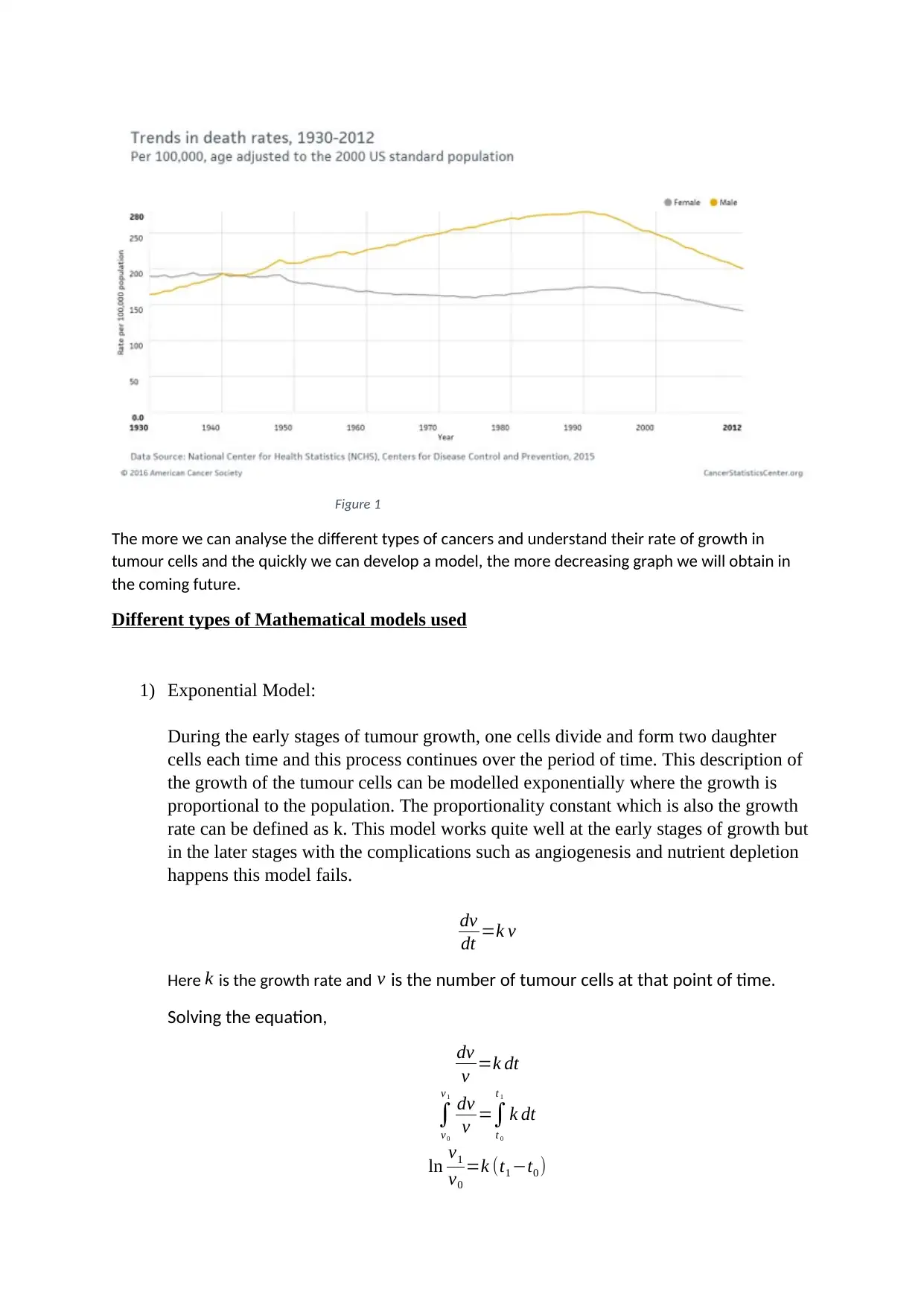
Figure 1
The more we can analyse the different types of cancers and understand their rate of growth in
tumour cells and the quickly we can develop a model, the more decreasing graph we will obtain in
the coming future.
Different types of Mathematical models used
1) Exponential Model:
During the early stages of tumour growth, one cells divide and form two daughter
cells each time and this process continues over the period of time. This description of
the growth of the tumour cells can be modelled exponentially where the growth is
proportional to the population. The proportionality constant which is also the growth
rate can be defined as k. This model works quite well at the early stages of growth but
in the later stages with the complications such as angiogenesis and nutrient depletion
happens this model fails.
dv
dt =k v
Here k is the growth rate and v is the number of tumour cells at that point of time.
Solving the equation,
dv
v =k dt
∫
v0
v1
dv
v =∫
t 0
t 1
k dt
ln v1
v0
=k (t1 −t0 )

v1 =v0 ek(t1−t 0)
This is the number of tumour cells present at the time instant t1.
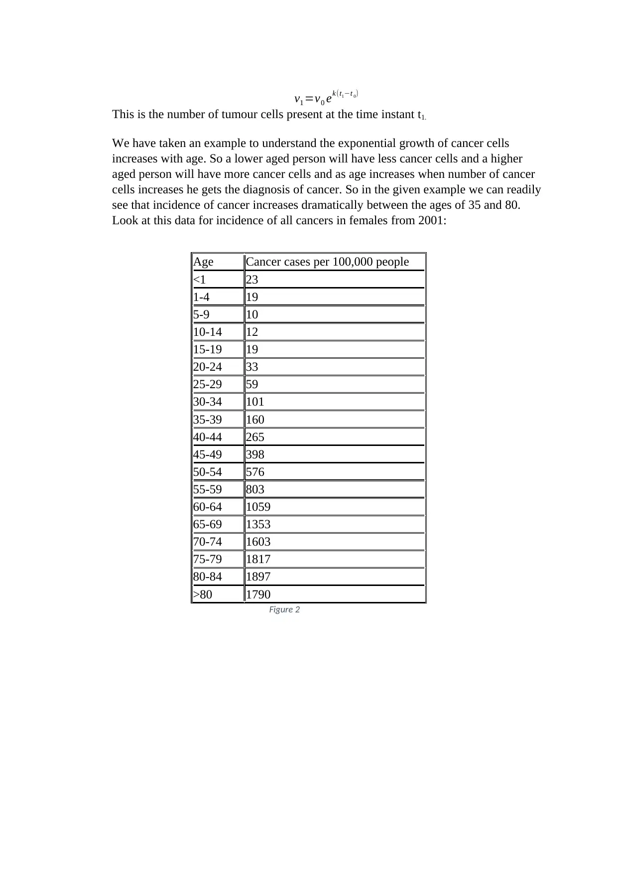
We have taken an example to understand the exponential growth of cancer cells
increases with age. So a lower aged person will have less cancer cells and a higher
aged person will have more cancer cells and as age increases when number of cancer
cells increases he gets the diagnosis of cancer. So in the given example we can readily
see that incidence of cancer increases dramatically between the ages of 35 and 80.
Look at this data for incidence of all cancers in females from 2001:
Age Cancer cases per 100,000 people
<1 23
1-4 19
5-9 10
10-14 12
15-19 19
20-24 33
25-29 59
30-34 101
35-39 160
40-44 265
45-49 398
50-54 576
55-59 803
60-64 1059
65-69 1353
70-74 1603
75-79 1817
80-84 1897
>80 1790
Figure 2

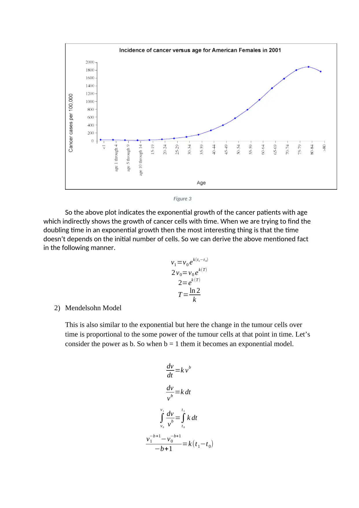
Figure 3
So the above plot indicates the exponential growth of the cancer patients with age
which indirectly shows the growth of cancer cells with time. When we are trying to find the
doubling time in an exponential growth then the most interesting thing is that the time
doesn’t depends on the initial number of cells. So we can derive the above mentioned fact
in the following manner.
v1 =v0 ek(t1−t 0)
2 v0=v0 ek(T)
2=ek (T)
T = ln 2
k
2) Mendelsohn Model
This is also similar to the exponential but here the change in the tumour cells over
time is proportional to the some power of the tumour cells at that point in time. Let’s
consider the power as b. So when b = 1 them it becomes an exponential model.
dv
dt =k vb
dv
vb =k dt
∫
v0
v1
dv
vb =∫
t 0
t 1
k dt
v1
−b +1−v0
−b+1
−b+1 =k (t1−t0)

v1
−b+1 =v0
−b +1 + (−b+1 )∗k (t1−t0 )
Now if we want to calculate the time at which the population becomes double we can
proceed with the following calculations.
2 v0
−b +1=v0
−b+ 1+ (−b+1 )∗k (t1−t0)
( 2−b +1−1 ) v0
−b +1
(−b+1 )∗k =T
Thus unlike exponential model this model the doubling time depends on the initial
population, b can take any value apart from 1.
3) Logistic Model
The differential equation of the model is:
dv
dt =k v∗(1− v
b )
In this model v describes the concentration of tumour cells in the body and dv
dt
describes the growth of a population over a time period dtthat is limited by a carrying
capacity of b. The growth rate is defined byk. From the equation we can interpret that
the equation growth rate decreases linearly with size and it becomes zero when the
concentration takes the value of the carrying capacity. If we do a double
differentiation we get the following equation
d2 v
d t2 =k2 v∗(1− v
b )∗(1− 2 v
b )
So it has a point of inflexion at the point b/2. If we solve the initial equation
dv
v∗(1− v
b )=k dt
bdv
v + dv
(1− v
b )
=k dt
Integrating this we get

b ln v−b∗ln (1− v
b )=k t
b ln v
(1− v
b )
=k t
ln v
(1− v
b )
= kt
b
v
(1− v
b )
=e
kt
b
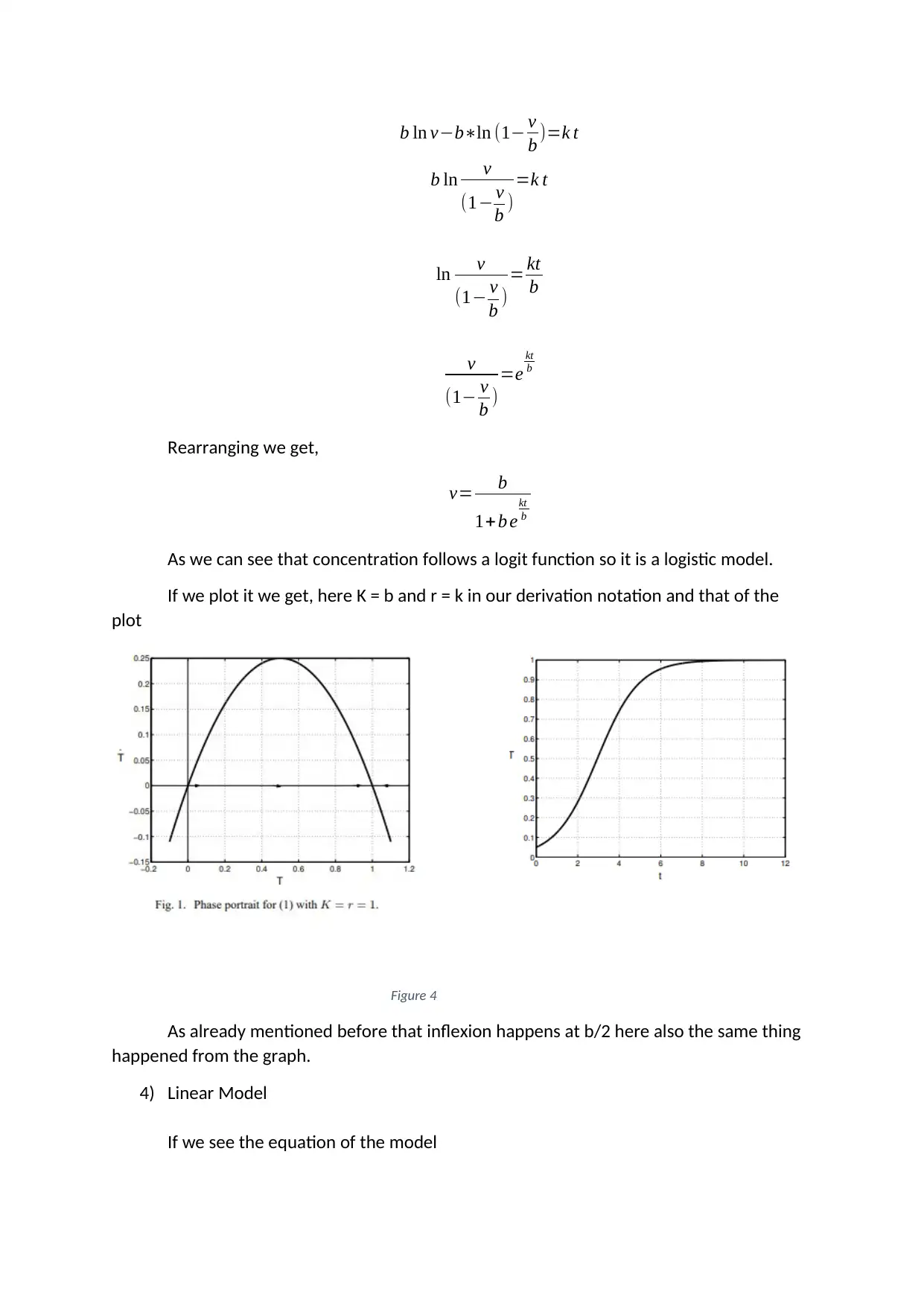
Rearranging we get,
v= b
1+ b e
kt
b
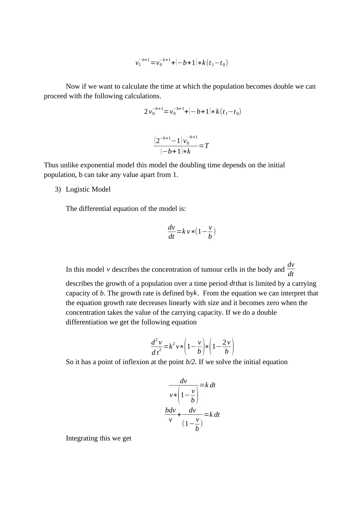
As we can see that concentration follows a logit function so it is a logistic model.
If we plot it we get, here K = b and r = k in our derivation notation and that of the
plot
Figure 4
As already mentioned before that inflexion happens at b/2 here also the same thing
happened from the graph.
4) Linear Model
If we see the equation of the model

dv
dt =k v /(v +b)Here initially the exponential growth rate is given by k/b but as it
reaches steady state then the growth rate becomes k. The model was used in early
research to analyse growth of cancer cell colonies.
Solving the differential equation,
(v+b) dv
v =k dt
(dv +b dv
v )=k dt
Integrating both sides
( v−v 0+ b ln v
v0
)=k (t−t0)
(ln ev−v0 +b ln v−b ln v0)=k (t−t0 )
¿
ev vb=e(v0+b ln v0 +k ( t −t0 ) )
ev vb=ev0
+ v0
b +ek (t −t0 )
So this can be solved with the help of numerical analysis.
5) Surface Model
In this model the surface of the tumour cell is expanding i.e. the surface of the tumour are
dividing whereas the cells inside the surface do nit reproduce so they are mitotically inactive.
The main idea is that in the early stage we are going to have the exponential growth and
later on it shifts to the secondary growth.
We can solve the equation with the help of partial fractions and integration by substitution
and finally with the help of numerical methods we can solve the problem.
dv
dt =k v /(v +b)
1
3
(v+ b)
1
3 dv
v =k dt

Let (v+b)
1
3 = z,
( v+ b ) =z3 ,
dv
dt =3 z2 dz
dt
v=z3−b
z 3 z2 dz
z3 −b =k dt
Now integrating on both the sides,
∫ z z2 dz
z3−b =∫ kdt
3
∫ ( 1+ b
z3 −b ) dz=∫ kdt
3
∫ dz+∫ b
z3−b dz=∫ kdt
3
z +b∫ 1
z3−(b1/ 3)3 dz =∫ kdt
3
Let ( b
1
3 )=a
z +b∫ 1
z3−a3 dz =∫ kdt
3
∫ 1
z3−a3 dz=∫ 1
( z−a)( z2+ az+a2) dz
1
( z−a)(z2 + az+a2)= A
z−a + Bz+C
( z2 +az +a2)
Solving for A, B and C we get the following,
A= 1
3 a , B=−1
3 a ∧C=−2/3
∫(
1
3 a
z −a +
−1
3 a z+−2
3
(z2+ az+a2 ) )dz
1
3 a ln ( z−a ) +∫
−1
3 a z +−2
3
(z2+ az +a2 ) dz

We can write the integral part as,
∫
−1
6 a (2 z +a)+−1
2
( z2+az +a2 ) dz
∫
−1
6 a (2 z+ a)
(z2 +az + a2) dz+∫
−1
2
( z2 +az + a2) dz
The first part will give
−1
6 a ln ( z2 +az +a2 )
And the second part becomes,
−1
2 ∫ 1
( z2+az +a2 ) dz
−1
2 ∫ 1
((z + a
2 )
2
+ 3 a2
4 )
dz
Let (z + a
2 ) = p
−1
2 ∫ 1
( p2 + 3 a2
4 )
dz
−1
2 tan−1
z + a
2
√ 3 a/2
−1
2 tan−1 2 z + a
√3 a
So finally solution becomes,
z +b ¿
(v+b)
1
3 +b ¿
So from the above solution v can be found out from the numerical analysis.

6) Bertalanffy Model
This model is supposed to be the best model to describe the growth of the tumour
cells. The best part is that it also takes account the cells which dies after sometime.
This model assumes that the growth is proportional to the surface area but there is
also a decrease in the concentration volume due to the death of the tumour cells.
dv
dt =k v
2
3 −b v
dv
dt +bv=k v
2
3
Dividing both the sides by v
2
3 ,we get,
dv
dt +bv=k v
2
3
v−2/ 3 dv
dt +b v1 /3=k
Let v
2
3 =z then v−2/ 3 dv
dt =3 dz
dt and substituting in the previous question,
3 dz
dt +bz=k
dz
dt + b
3 z= k
3
Now the Integrating factor is e∫ b
3 dt and multiplying it on both the sides
e∫ b
3 dt
( dz
dt + b
3 z )= k
3 e∫ b
3 dt
d ( e
b
3 t
z ) = k
3 e
b
3 t
dt
Now integrating both the sides we get,
z= k
b t+c e
−b
3 t

Where c is a constant now substituting z with the previous value v
2
3 =z
We get,
v=( k
b t+ c e
−b
3 t
)
3 /2
So you can see in the final expression it increases as well as decreases. This model is the
best to describe the human tumour.
7) Gompertz Model
This model is similar to the logistics model but the only difference is that the in this
model about the inflexion point it is not symmetric but whereas in case of the
logistics model it is symmetric. This model provides the best fit for breast and lung
cancer growth. We can write the equation of the model as
dv
dt =k v∗ln b
v +c
It can be simplified as dv
dt =k v∗¿
Now dividing by v and rearranging we get,
1
v
dv
dt +kb ln v=ka
Now let us consider, ln v=z, 1
v
dv
dt = dz
dt we can write the above equation as,
dz
dt +kbz=ka
Now the Integrating factor is e∫kb dt and multiplying it on both the sides
e∫kb dt ( dz
dt + kbz)=ka e∫kbdt
d ( ekbt z )=ka ekbt dt
Now integrating both the sides,
z= a
b t +c e−kbt

Where c is a constant.
This above mentioned seven methodologies are used for the modelling the concentration of
tumour cells in the human body as well as finding the rate of growth of them in our body.
The model which we fit is we can test the goodness of fit by the Sum of squares of residuals
but since it has so many parameters it is not the fair way as it can give less bias but increase
the variance always so we can go for Aikaike’s information criterion (AICC), which is generally
used for small sample size. The AICC is given by
AICc=n ln SSR
n + 2 ( K +1 ) n
n−K−2
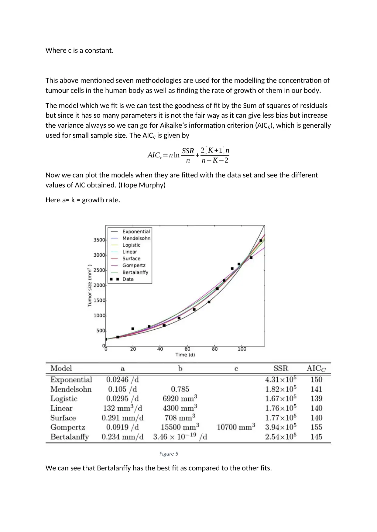
Now we can plot the models when they are fitted with the data set and see the different
values of AIC obtained. (Hope Murphy)
Here a= k = growth rate.
Figure 5
We can see that Bertalanffy has the best fit as compared to the other fits.