Mathematical Modelling in Aerospace Engineering Project - Coventry Uni
VerifiedAdded on 2022/11/23
|9
|1858
|201
Project
AI Summary
This document presents a comprehensive solution to a mathematical modelling project in aerospace engineering. It begins with an explanation of mechanistic and data-driven modelling approaches, highlighting their differences and applications in aerospace. The solution then delves into interpolation and regression techniques, providing practical examples. The core of the assignment involves solving several problems: calculating loan repayments using the EMI formula, modelling a falling object using data-driven differential equation techniques and MATLAB code, and applying cubic splines to analyze velocimeter data from a parachutist problem. The document includes detailed calculations, MATLAB code, and graphical representations to illustrate the concepts and solutions, providing a thorough understanding of mathematical modelling in aerospace engineering.
Running head: MATHEMATICAL MODELLING IN AEROSPACE ENGINEERING
MATHEMATICAL MODELLING IN AEROSPACE ENGINEERING
Name of the Student
Name of the University
Author Note
MATHEMATICAL MODELLING IN AEROSPACE ENGINEERING
Name of the Student
Name of the University
Author Note
Paraphrase This Document
Need a fresh take? Get an instant paraphrase of this document with our AI Paraphraser
1MATHEMATICAL MODELLING IN AEROSPACE ENGINEERING
Q1: Mechanistic and Data-Driven Modelling
A mechanistic model is described by a differential equation of reaction or process rate. The
model is usually represented by a stoichiometric matrix by which one component type is
converted to another component type, satisfying the conservation mass, energy, net power
flow or elements. The mass balance is described in a mechanistic model by which flows are
represented at the system boundaries.
A data driven model is usually described in an equation format with different levels of
complexity as per the data (like exponential model or polynomial model of some order). The
technique of regression is commonly used in a data driven model where any given data is
fitted with simple to complex equations within desired level of error.
The difference between a mechanistic model and data driven model is that in a mechanistic
model the differential equation is established by laws of physics, chemistry and logical
mathematics, whereas in case of data driven model the equations are formed by applying
statistical methods without inspection of physical relationship between the variables (Dalmau
et al. 2015). A mechanistic model does not depend on any collected data about the variable,
instead data can be generated from the mechanistic model. Validity of Data driven or
statistical model entirely depends of collected data even if proper statistical techniques with
low significance level has been applied to generate the model. A mechanistic model is always
valid if all the variables are taken into account and proper logical relationship is obtained.
However, a data driven model cannot be entirely accurate as probabilistic methods are used
and in real cases there is always some error in model (Remesan and Mathew 2016).
Sometimes generating a mechanistic model can be troublesome and time consuming due to
complexity of analytical solutions or for unknown relationships between variables, whereas
data driven model can always be fitted to data with data points of available variables by
probabilistic methods.
The Mechanistic models are extensively used in aerospace engineering and applications in
the fields of flight dynamics, space technology and aerospace structure formulation and in
other aerospace related topics. The data driven models are used in anomaly detection of
aircraft and spacecraft by which faults and failures in complex aerospace systems. Also, data
driven regression models can be used to predict the power and fuel consumption of a
spacecraft.
Q2: Interpolation
Interpolation is mathematical method of constructing new data points within a set of known
discrete data points (Dehghan, Abbaszadeh and Mohebbi 2016). The different interpolation
techniques are Piecewise constant interpolation, linear interpolation, polynomial interpolation
and spline interpolation.
Q3: Regression
Regression is a statistical analysis technique by which some mathematical relationship is
established between a dependent and independent variables. Regression is used to predict
value of target variable at some unknown points of independent variables (Castro and
Pereira-Filho 2016). The different regression types are linear regression, polynomial
regression, Ridge regression, Lasso regression and Elastic regression.

2MATHEMATICAL MODELLING IN AEROSPACE ENGINEERING
P1: Single-Rate Loan Repayment
Here, T = 256 months and r = 0.33% per month.
Principle borrow amount (P) = £1,500,000
a) The amount that is needed to be paid per month such that completely debt relief after T
months is given by the EMI formula
EMI= P∗r∗( 1+r )T
( 1+ r )T −1 = 1,500,000∗0.0033∗( 1+0.0033 ) 256
( 1+ 0.0033 ) 256 – 1 = £ 8687.89.
Hence, £ 495000 is needed to be paid per month to become completely debt free after T =
256 months when same amount is paid in every month and monthly interest is applied to the
outstanding balance by a monthly basis.
b) The amount outstanding after N months can be calculated by the following formula
Amount = P ( 1+ r ) N – a ( 1+r ) N−1 – a ( 1+r ) N−2−…−a ( 1+r ) −a
Where a = EMI paid after each month = £ 8687.89
= P ( 1+ r )128 – a (1+ r )127 – a (1+r )126−…−a (1+ r )
= P ( 1+ r ) 128 – ¿
= 1500000 ( 1+0.0033 ) 128 – ¿
= 1500000 ( 1.0033 ) 128 – ( 495000∗( 1.0033128 – 1 )
0.0033 )
= £ 905836.60
Hence, the outstanding balance after 128 months is £ 905836.60 when the EMI is paid for
128 months.
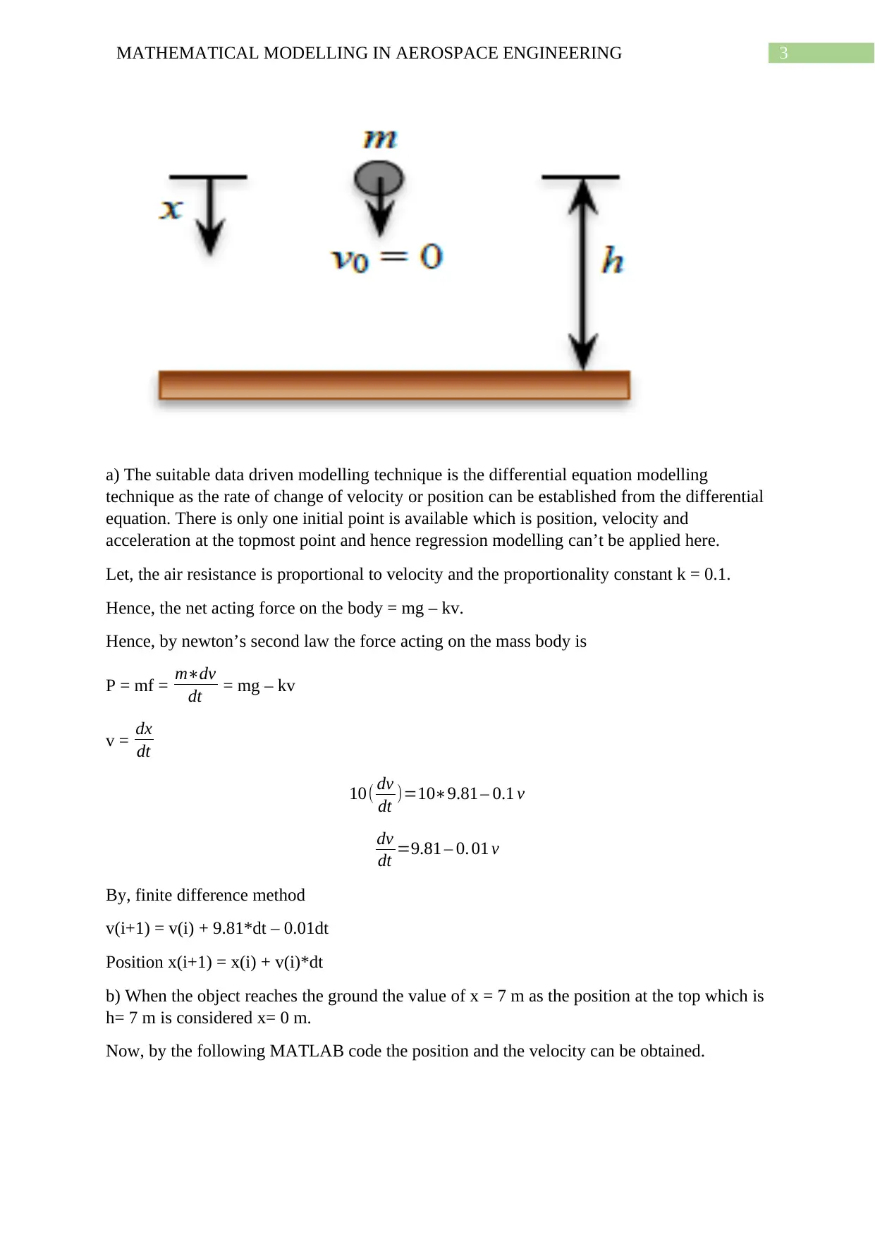
P2: Data-Driven Modelling of Falling Object
The mass of the object is m = 10 kg which falls from the height h = 7 m. The initial velocity
and initial acceleration are v0 = 0 m/s and g=9.81 m
s2 . The schematic diagram of the problem
is given below.
P1: Single-Rate Loan Repayment
Here, T = 256 months and r = 0.33% per month.
Principle borrow amount (P) = £1,500,000
a) The amount that is needed to be paid per month such that completely debt relief after T
months is given by the EMI formula
EMI= P∗r∗( 1+r )T
( 1+ r )T −1 = 1,500,000∗0.0033∗( 1+0.0033 ) 256
( 1+ 0.0033 ) 256 – 1 = £ 8687.89.
Hence, £ 495000 is needed to be paid per month to become completely debt free after T =
256 months when same amount is paid in every month and monthly interest is applied to the
outstanding balance by a monthly basis.
b) The amount outstanding after N months can be calculated by the following formula
Amount = P ( 1+ r ) N – a ( 1+r ) N−1 – a ( 1+r ) N−2−…−a ( 1+r ) −a
Where a = EMI paid after each month = £ 8687.89
= P ( 1+ r )128 – a (1+ r )127 – a (1+r )126−…−a (1+ r )
= P ( 1+ r ) 128 – ¿
= 1500000 ( 1+0.0033 ) 128 – ¿
= 1500000 ( 1.0033 ) 128 – ( 495000∗( 1.0033128 – 1 )
0.0033 )
= £ 905836.60
Hence, the outstanding balance after 128 months is £ 905836.60 when the EMI is paid for
128 months.
P2: Data-Driven Modelling of Falling Object
The mass of the object is m = 10 kg which falls from the height h = 7 m. The initial velocity
and initial acceleration are v0 = 0 m/s and g=9.81 m
s2 . The schematic diagram of the problem
is given below.
⊘ This is a preview!⊘
Do you want full access?
Subscribe today to unlock all pages.
Trusted by 1+ million students worldwide
3MATHEMATICAL MODELLING IN AEROSPACE ENGINEERING
a) The suitable data driven modelling technique is the differential equation modelling
technique as the rate of change of velocity or position can be established from the differential
equation. There is only one initial point is available which is position, velocity and
acceleration at the topmost point and hence regression modelling can’t be applied here.
Let, the air resistance is proportional to velocity and the proportionality constant k = 0.1.
Hence, the net acting force on the body = mg – kv.
Hence, by newton’s second law the force acting on the mass body is
P = mf = m∗dv
dt = mg – kv
v = dx
dt
10( dv
dt )=10∗9.81 – 0.1 v
dv
dt =9.81 – 0. 01 v
By, finite difference method
v(i+1) = v(i) + 9.81*dt – 0.01dt
Position x(i+1) = x(i) + v(i)*dt
b) When the object reaches the ground the value of x = 7 m as the position at the top which is
h= 7 m is considered x= 0 m.
Now, by the following MATLAB code the position and the velocity can be obtained.
Paraphrase This Document
Need a fresh take? Get an instant paraphrase of this document with our AI Paraphraser

4MATHEMATICAL MODELLING IN AEROSPACE ENGINEERING
MATLAB code:
t = linspace(0,1.5,150);
dt = t(2) - t(1);
v(1) = 0; g = 9.81; k= 0.1; m=10;
for i=1:length(t)
v(i+1) = v(i) + g*dt - (k/m)*dt;
end
x(1) = 0;
for i=1:length(t)
x(i+1) = x(i) + v(i)*dt;
end
figure(1)
subplot(2,1,1)
plot(t,x(1:end-1))
title('height from the top x=0 in meters')
xlabel('Time t in secs')
ylabel('Position')
grid on
ylim([0 8])
subplot(2,1,2)
plot(t,v(1:end-1))
title('velocity of the object in m/sec')
xlabel('Time t in secs')
ylabel('velocity')
grid on
xlim([0 1.2])
5MATHEMATICAL MODELLING IN AEROSPACE ENGINEERING
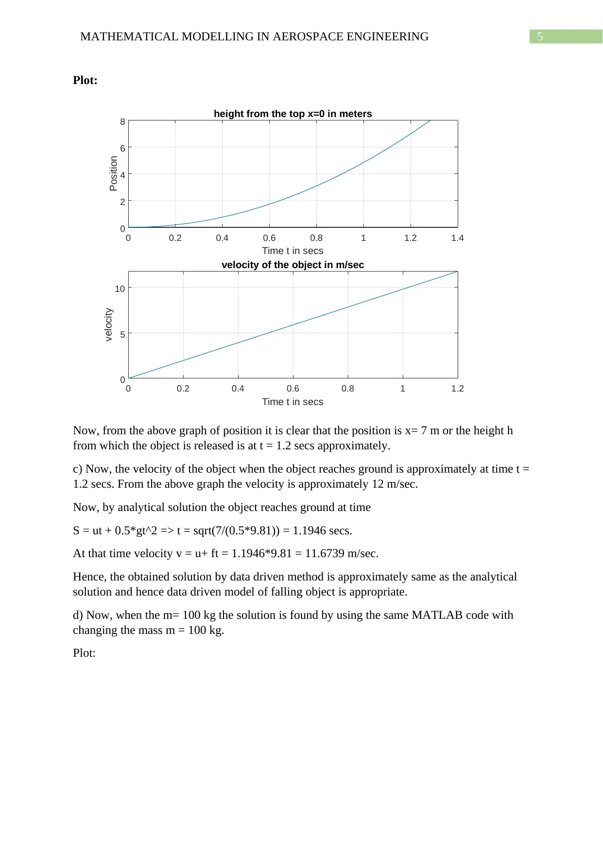
Plot:
0 0.2 0.4 0.6 0.8 1 1.2 1.4
Time t in secs
0
2
4
6
8
Position
height from the top x=0 in meters
0 0.2 0.4 0.6 0.8 1 1.2
Time t in secs
0
5
10
velocity
velocity of the object in m/sec
Now, from the above graph of position it is clear that the position is x= 7 m or the height h
from which the object is released is at t = 1.2 secs approximately.
c) Now, the velocity of the object when the object reaches ground is approximately at time t =
1.2 secs. From the above graph the velocity is approximately 12 m/sec.
Now, by analytical solution the object reaches ground at time
S = ut + 0.5*gt^2 => t = sqrt(7/(0.5*9.81)) = 1.1946 secs.
At that time velocity v = u+ ft = 1.1946*9.81 = 11.6739 m/sec.
Hence, the obtained solution by data driven method is approximately same as the analytical
solution and hence data driven model of falling object is appropriate.
d) Now, when the m= 100 kg the solution is found by using the same MATLAB code with
changing the mass m = 100 kg.
Plot:
Plot:
0 0.2 0.4 0.6 0.8 1 1.2 1.4
Time t in secs
0
2
4
6
8
Position
height from the top x=0 in meters
0 0.2 0.4 0.6 0.8 1 1.2
Time t in secs
0
5
10
velocity
velocity of the object in m/sec
Now, from the above graph of position it is clear that the position is x= 7 m or the height h
from which the object is released is at t = 1.2 secs approximately.
c) Now, the velocity of the object when the object reaches ground is approximately at time t =
1.2 secs. From the above graph the velocity is approximately 12 m/sec.
Now, by analytical solution the object reaches ground at time
S = ut + 0.5*gt^2 => t = sqrt(7/(0.5*9.81)) = 1.1946 secs.
At that time velocity v = u+ ft = 1.1946*9.81 = 11.6739 m/sec.
Hence, the obtained solution by data driven method is approximately same as the analytical
solution and hence data driven model of falling object is appropriate.
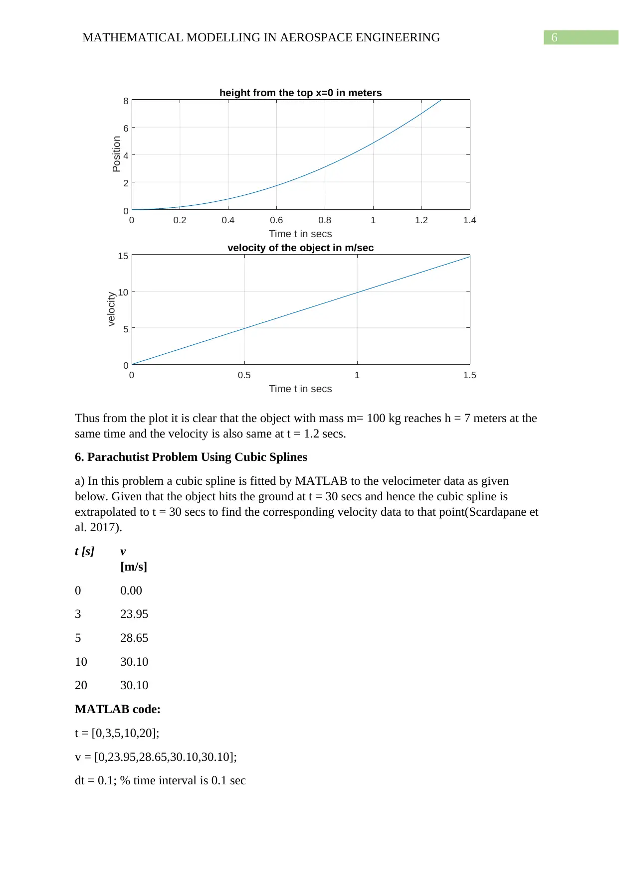
d) Now, when the m= 100 kg the solution is found by using the same MATLAB code with
changing the mass m = 100 kg.
Plot:
⊘ This is a preview!⊘
Do you want full access?
Subscribe today to unlock all pages.
Trusted by 1+ million students worldwide
6MATHEMATICAL MODELLING IN AEROSPACE ENGINEERING
0 0.2 0.4 0.6 0.8 1 1.2 1.4
Time t in secs
0
2
4
6
8
Position
height from the top x=0 in meters
0 0.5 1 1.5
Time t in secs
0
5
10
15
velocity
velocity of the object in m/sec
Thus from the plot it is clear that the object with mass m= 100 kg reaches h = 7 meters at the
same time and the velocity is also same at t = 1.2 secs.
6. Parachutist Problem Using Cubic Splines
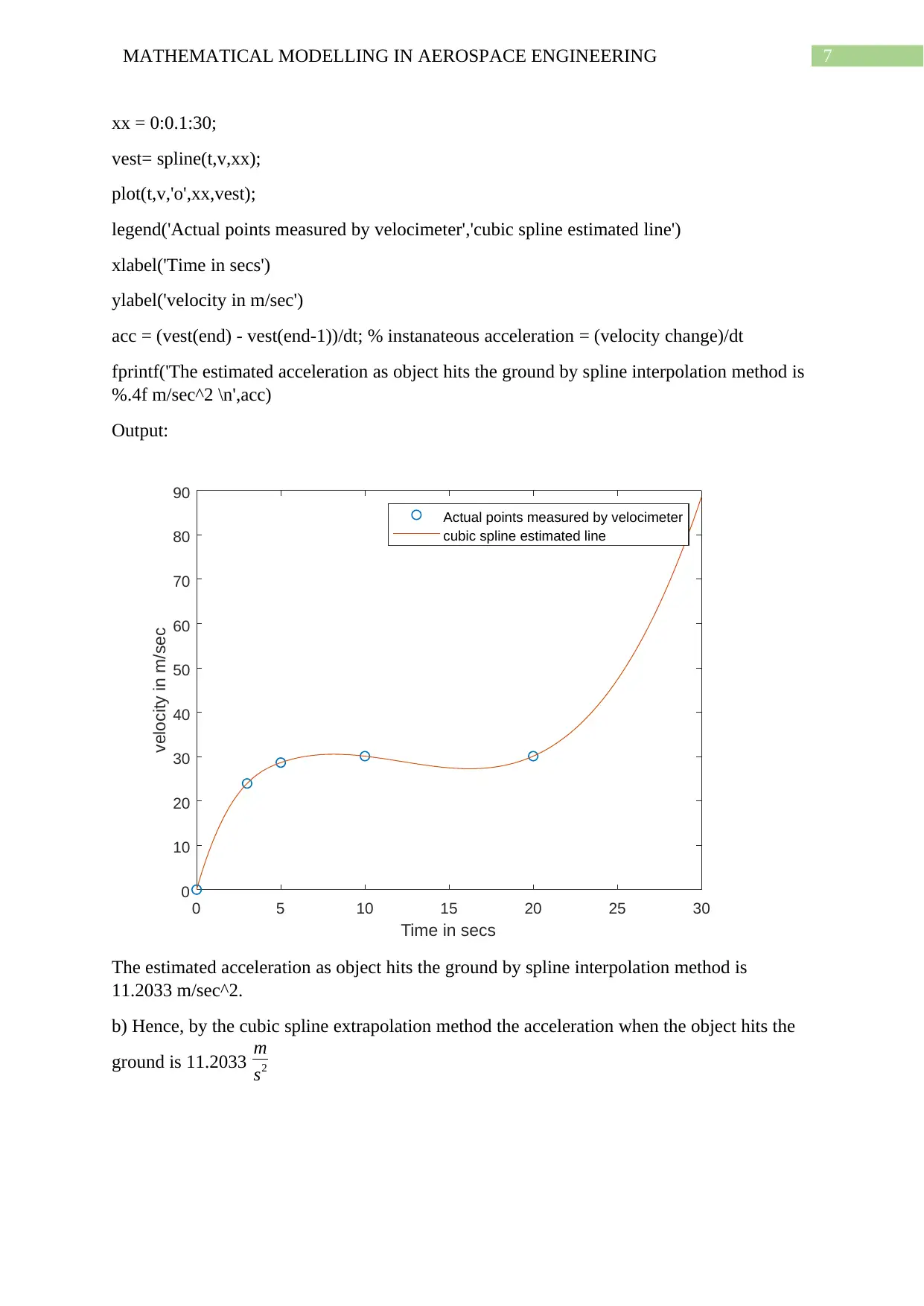
a) In this problem a cubic spline is fitted by MATLAB to the velocimeter data as given
below. Given that the object hits the ground at t = 30 secs and hence the cubic spline is
extrapolated to t = 30 secs to find the corresponding velocity data to that point(Scardapane et
al. 2017).
t [s] v
[m/s]
0 0.00
3 23.95
5 28.65
10 30.10
20 30.10
MATLAB code:
t = [0,3,5,10,20];
v = [0,23.95,28.65,30.10,30.10];
dt = 0.1; % time interval is 0.1 sec
0 0.2 0.4 0.6 0.8 1 1.2 1.4
Time t in secs
0
2
4
6
8
Position
height from the top x=0 in meters
0 0.5 1 1.5
Time t in secs
0
5
10
15
velocity
velocity of the object in m/sec
Thus from the plot it is clear that the object with mass m= 100 kg reaches h = 7 meters at the
same time and the velocity is also same at t = 1.2 secs.
6. Parachutist Problem Using Cubic Splines
a) In this problem a cubic spline is fitted by MATLAB to the velocimeter data as given
below. Given that the object hits the ground at t = 30 secs and hence the cubic spline is
extrapolated to t = 30 secs to find the corresponding velocity data to that point(Scardapane et
al. 2017).
t [s] v
[m/s]
0 0.00
3 23.95
5 28.65
10 30.10
20 30.10
MATLAB code:
t = [0,3,5,10,20];
v = [0,23.95,28.65,30.10,30.10];
dt = 0.1; % time interval is 0.1 sec
Paraphrase This Document
Need a fresh take? Get an instant paraphrase of this document with our AI Paraphraser
7MATHEMATICAL MODELLING IN AEROSPACE ENGINEERING
xx = 0:0.1:30;
vest= spline(t,v,xx);
plot(t,v,'o',xx,vest);
legend('Actual points measured by velocimeter','cubic spline estimated line')
xlabel('Time in secs')
ylabel('velocity in m/sec')
acc = (vest(end) - vest(end-1))/dt; % instanateous acceleration = (velocity change)/dt
fprintf('The estimated acceleration as object hits the ground by spline interpolation method is
%.4f m/sec^2 \n',acc)
Output:
0 5 10 15 20 25 30
Time in secs
0
10
20
30
40
50
60
70
80
90
velocity in m/sec
Actual points measured by velocimeter
cubic spline estimated line
The estimated acceleration as object hits the ground by spline interpolation method is
11.2033 m/sec^2.
b) Hence, by the cubic spline extrapolation method the acceleration when the object hits the
ground is 11.2033 m
s2
8MATHEMATICAL MODELLING IN AEROSPACE ENGINEERING
References:
Dalmau, M., Atanasova, N., Gabarrón, S., Rodriguez-Roda, I. and Comas, J., 2015.
Comparison of a deterministic and a data driven model to describe MBR fouling. Chemical
Engineering Journal, 260, pp.300-308.
Remesan, R. and Mathew, J., 2016. Hydrological data driven modelling. Springer
International Pu.
Castro, J.P. and Pereira-Filho, E.R., 2016. Twelve different types of data normalization for
the proposition of classification, univariate and multivariate regression models for the direct
analyses of alloys by laser-induced breakdown spectroscopy (LIBS). Journal of Analytical
Atomic Spectrometry, 31(10), pp.2005-2014.
Dehghan, M., Abbaszadeh, M. and Mohebbi, A., 2016. The use of element free Galerkin
method based on moving Kriging and radial point interpolation techniques for solving some
types of Turing models. Engineering Analysis with Boundary Elements, 62, pp.93-111.
Scardapane, S., Scarpiniti, M., Comminiello, D. and Uncini, A., 2017, June. Learning
activation functions from data using cubic spline interpolation. In Italian Workshop on
Neural Nets(pp. 73-83). Springer, Cham.
⊘ This is a preview!⊘
Do you want full access?
Subscribe today to unlock all pages.
Trusted by 1+ million students worldwide
1 out of 9

Your All-in-One AI-Powered Toolkit for Academic Success.
+13062052269
info@desklib.com
Available 24*7 on WhatsApp / Email
![[object Object]](/_next/static/media/star-bottom.7253800d.svg)
Unlock your academic potential
Copyright © 2020–2026 A2Z Services. All Rights Reserved. Developed and managed by ZUCOL.