Mathematical Modelling (Maths): SIS Model Analysis and Solutions

This assignment analyzes the Susceptible-Infected-Susceptible (SIS) model, a mathematical model used to simulate the spread of infectious diseases. It begins with an explanation of the SIS model, its equations (dS/dt = γI – βSI and dI/dt = βSI – γI), and the parameters involved, including the infectious contact rate (β) and the recovery rate (γ). The document explores the stiffness of the equations and the impact of step size on numerical solutions. The solution employs the Runge-Kutta method and derives both numerical and analytical solutions for the model. The analysis includes the derivation of equations for the infected population (I) and susceptible population (S), considering a constant total population (N). It also discusses the equilibrium conditions (dS/dt = 0, dI/dt = 0) and the stability of the system, relating the infection rate to the recovery rate. The document concludes by highlighting the relationship between parameter values (β, γ) and the infected population (I), and the simulation of the spread of an infection in a population of 1 million.

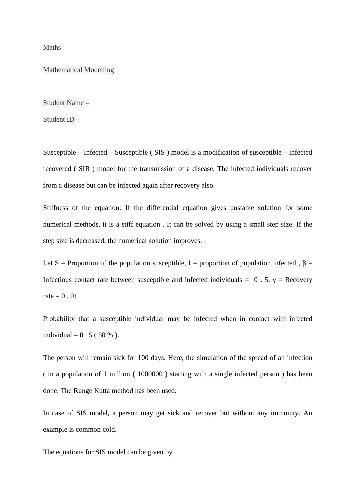
Maths
Mathematical Modelling
Student Name –
Student ID –
Susceptible – Infected – Susceptible ( SIS ) model is a modification of susceptible – infected
recovered ( SIR ) model for the transmission of a disease. The infected individuals recover
from a disease but can be infected again after recovery also.
Stiffness of the equation: If the differential equation gives unstable solution for some
numerical methods, it is a stiff equation . It can be solved by using a small step size. If the
step size is decreased, the numerical solution improves.
Let S = Proportion of the population susceptible, I = proportion of population infected , β =
Infectious contact rate between susceptible and infected individuals = 0 . 5, γ = Recovery
rate = 0 . 01
Probability that a susceptible individual may be infected when in contact with infected
individual = 0 . 5 ( 50 % ).
The person will remain sick for 100 days. Here, the simulation of the spread of an infection
( in a population of 1 million ( 1000000 ) starting with a single infected person ) has been
done. The Runge Kutta method has been used.
In case of SIS model, a person may get sick and recover but without any immunity. An
example is common cold.
The equations for SIS model can be given by

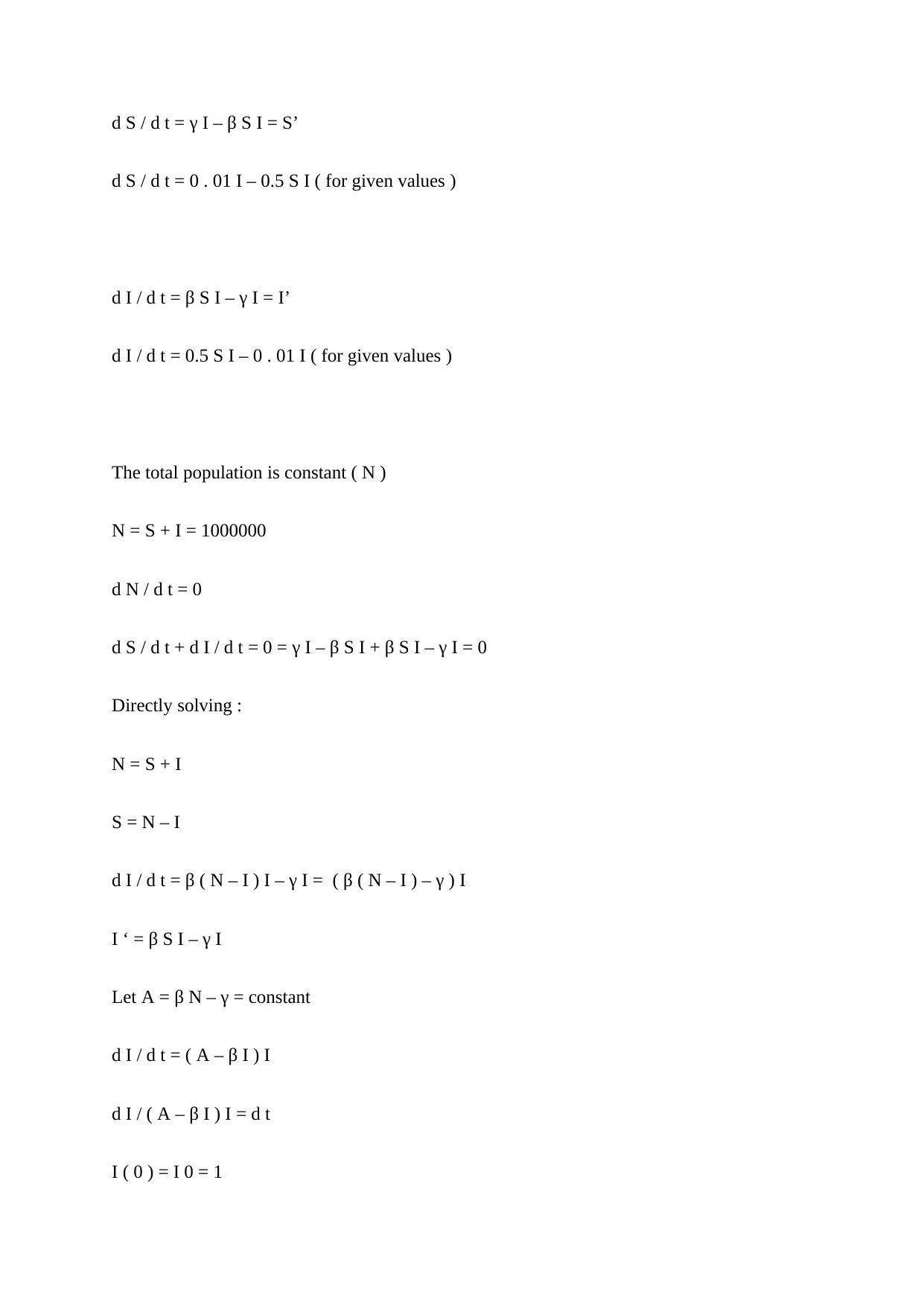
d S / d t = γ I – β S I = S’
d S / d t = 0 . 01 I – 0.5 S I ( for given values )
d I / d t = β S I – γ I = I’
d I / d t = 0.5 S I – 0 . 01 I ( for given values )
The total population is constant ( N )
N = S + I = 1000000
d N / d t = 0
d S / d t + d I / d t = 0 = γ I – β S I + β S I – γ I = 0
Directly solving :
N = S + I
S = N – I
d I / d t = β ( N – I ) I – γ I = ( β ( N – I ) – γ ) I
I ‘ = β S I – γ I
Let A = β N – γ = constant
d I / d t = ( A – β I ) I
d I / ( A – β I ) I = d t
I ( 0 ) = I 0 = 1

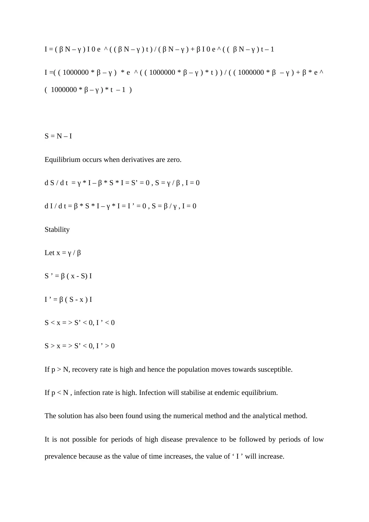
I = ( β N – γ ) I 0 e ^ ( ( β N – γ ) t ) / ( β N – γ ) + β I 0 e ^ ( ( β N – γ ) t – 1
I =( ( 1000000 * β – γ ) * e ^ ( ( 1000000 * β – γ ) * t ) ) / ( ( 1000000 * β – γ ) + β * e ^
( 1000000 * β – γ ) * t – 1 )
S = N – I
Equilibrium occurs when derivatives are zero.
d S / d t = γ * I – β * S * I = S’ = 0 , S = γ / β , I = 0
d I / d t = β * S * I – γ * I = I ’ = 0 , S = β / γ , I = 0
Stability
Let x = γ / β
S ’ = β ( x - S) I
I ’ = β ( S - x ) I
S < x = > S’ < 0, I ’ < 0
S > x = > S’ < 0, I ’ > 0
If p > N, recovery rate is high and hence the population moves towards susceptible.
If p < N , infection rate is high. Infection will stabilise at endemic equilibrium.
The solution has also been found using the numerical method and the analytical method.
It is not possible for periods of high disease prevalence to be followed by periods of low
prevalence because as the value of time increases, the value of ‘ I ’ will increase.

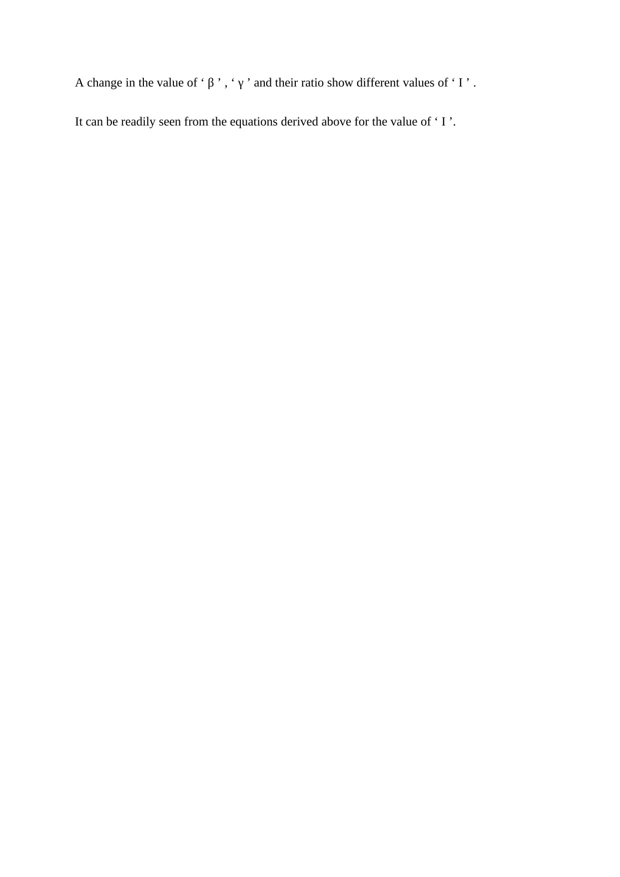
A change in the value of ‘ β ’ , ‘ γ ’ and their ratio show different values of ‘ I ’ .
It can be readily seen from the equations derived above for the value of ‘ I ’.