Statistical Concepts and Applications Assignment - Semester 1

This document presents a comprehensive solution to a statistics assignment focusing on mathematical concepts and statistical applications. The assignment covers several key areas, including normal distribution, sampling distributions, the central limit theorem, binomial distributions, and the normal approximation to binomial distributions. The solution provides step-by-step calculations and explanations for problems related to the height of females, gestation periods, calorie intake of males, oil changes, and fishing catch rates. It also addresses problems related to new product failures in grocery stores. The solutions utilize Z-scores, probability calculations, and continuity correction factors to arrive at the final answers. The document demonstrates the application of statistical concepts to real-world scenarios and provides a detailed analysis of each problem.

Mathematical Concepts and Statistical Applications
Mathematics Application
Student Name
Institution Affiliation

Mathematical Concepts and Statistical Applications
Normal Distribution – Sampling Distributions – Central Limit Theorem
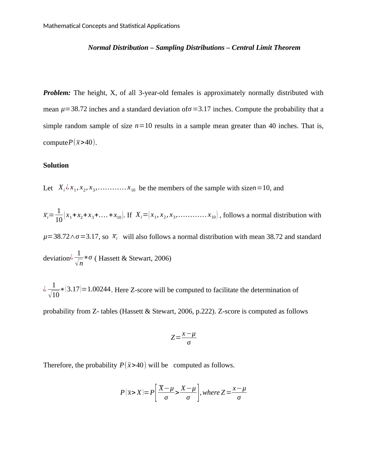
Problem: The height, X, of all 3-year-old females is approximately normally distributed with
mean μ=38.72 inches and a standard deviation of σ =3.17 inches. Compute the probability that a
simple random sample of size n=10 results in a sample mean greater than 40 inches. That is,
computeP( x >40).
Solution
Let Xi ¿ x1 , x2 , x3 , …… … … x10 be the members of the sample with size n=10, and
xi= 1
10 ( x1 +x2 +x3 +… . + x10 ). If Xi = ( x1 , x2 , x3 , … … … … x10 ) , follows a normal distribution with
μ=38.72∧σ =3.17, so xi will also follows a normal distribution with mean 38.72 and standard
deviation¿ 1
√n∗σ ( Hassett & Stewart, 2006)
¿ 1
√ 10∗ ( 3.17 ) =1.00244. Here Z-score will be computed to facilitate the determination of
probability from Z- tables (Hassett & Stewart, 2006, p.222). Z-score is computed as follows
Z= x −μ
σ
Therefore, the probability P( x >40) will be computed as follows.
P ( x> X ) =P [ X−μ
σ > X −μ
σ ] , where Z = x−μ
σ

Mathematical Concepts and Statistical Applications
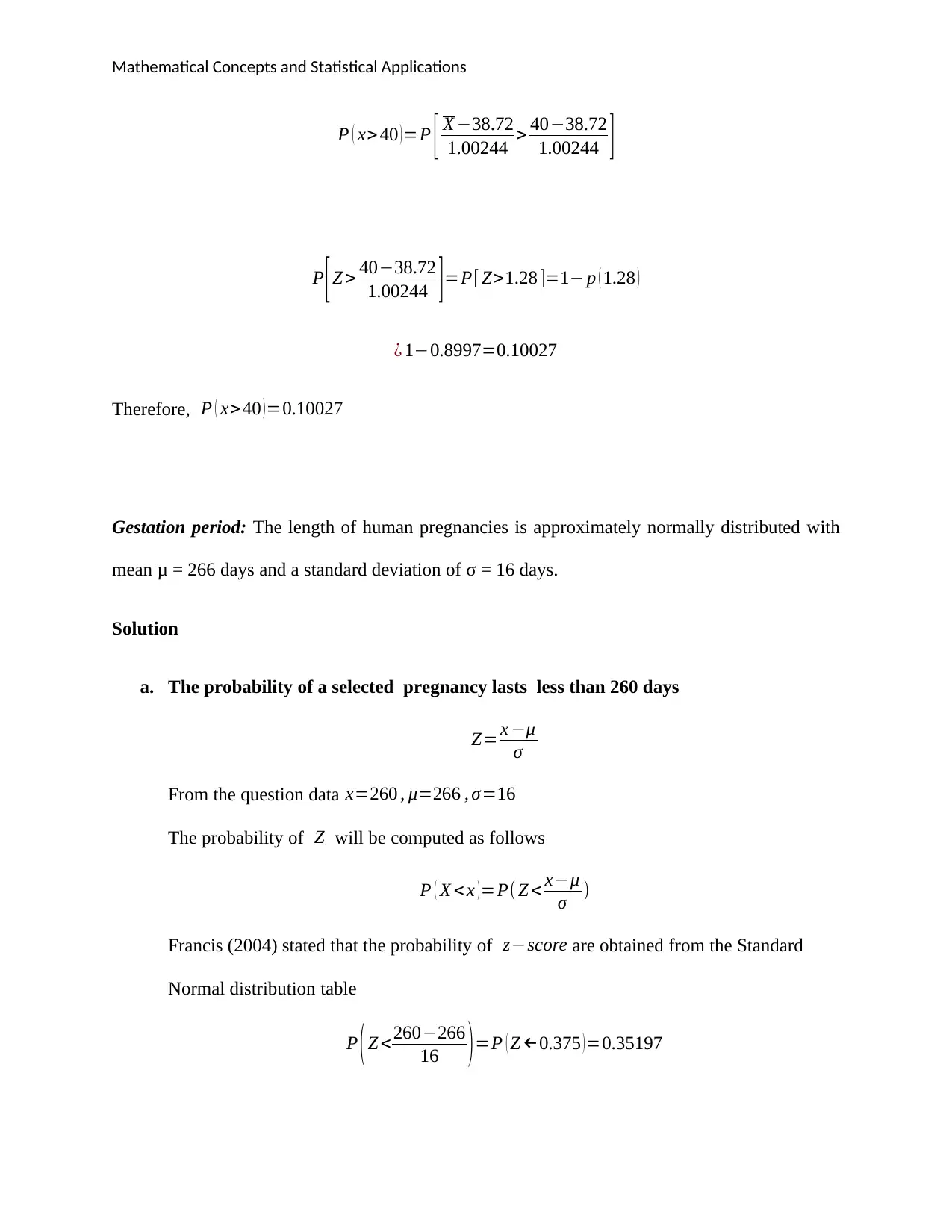
P ( x>40 )=P [ X −38.72
1.00244 > 40−38.72
1.00244 ]
P [Z > 40−38.72
1.00244 ]=P[ Z>1.28 ]=1− p ( 1.28 )
¿ 1−0.8997=0.10027
Therefore, P ( x>40 )=0.10027
Gestation period: The length of human pregnancies is approximately normally distributed with
mean μ = 266 days and a standard deviation of σ = 16 days.
Solution
a. The probability of a selected pregnancy lasts less than 260 days
Z= x −μ
σ
From the question data x=260 , μ=266 , σ=16
The probability of Z will be computed as follows
P ( X < x )=P( Z < x−μ
σ )
Francis (2004) stated that the probability of z−score are obtained from the Standard
Normal distribution table
P (Z < 260−266
16 )=P ( Z ←0.375 )=0.35197

Mathematical Concepts and Statistical Applications
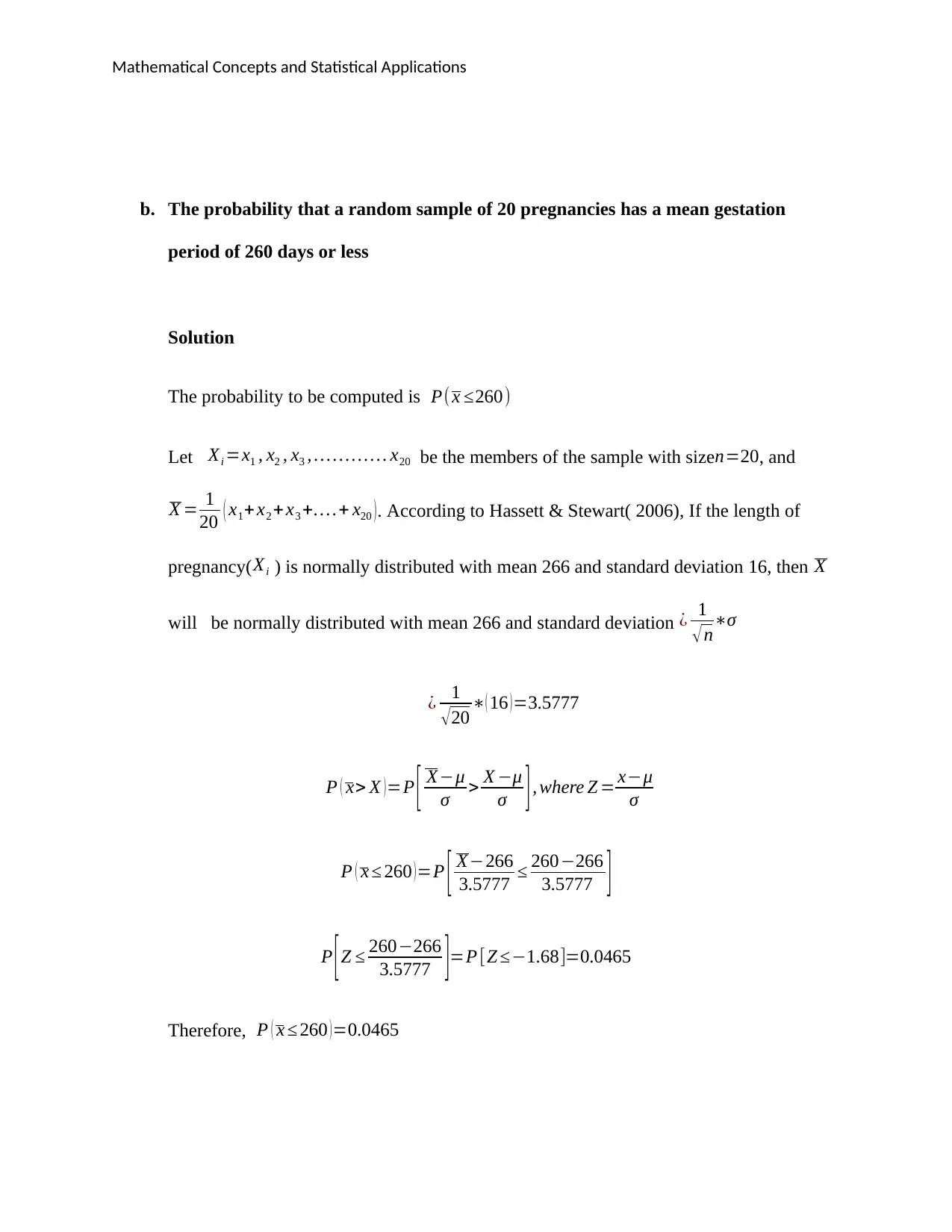
b. The probability that a random sample of 20 pregnancies has a mean gestation
period of 260 days or less
Solution
The probability to be computed is P( x ≤260)
Let Xi =x1 , x2 , x3 , … … … … x20 be the members of the sample with sizen=20, and
X = 1
20 ( x1+ x2 + x3 +… .+ x20 ). According to Hassett & Stewart( 2006), If the length of
pregnancy(Xi ) is normally distributed with mean 266 and standard deviation 16, then X
will be normally distributed with mean 266 and standard deviation ¿ 1
√ n∗σ
¿ 1
√ 20 ∗( 16 ) =3.5777
P ( x> X ) =P [ X−μ
σ > X −μ
σ ] , where Z = x−μ
σ
P ( x ≤ 260 )=P [ X−266
3.5777 ≤ 260−266
3.5777 ]
P [ Z ≤ 260−266
3.5777 ]=P [Z ≤−1.68]=0.0465
Therefore, P ( x ≤ 260 ) =0.0465

Mathematical Concepts and Statistical Applications
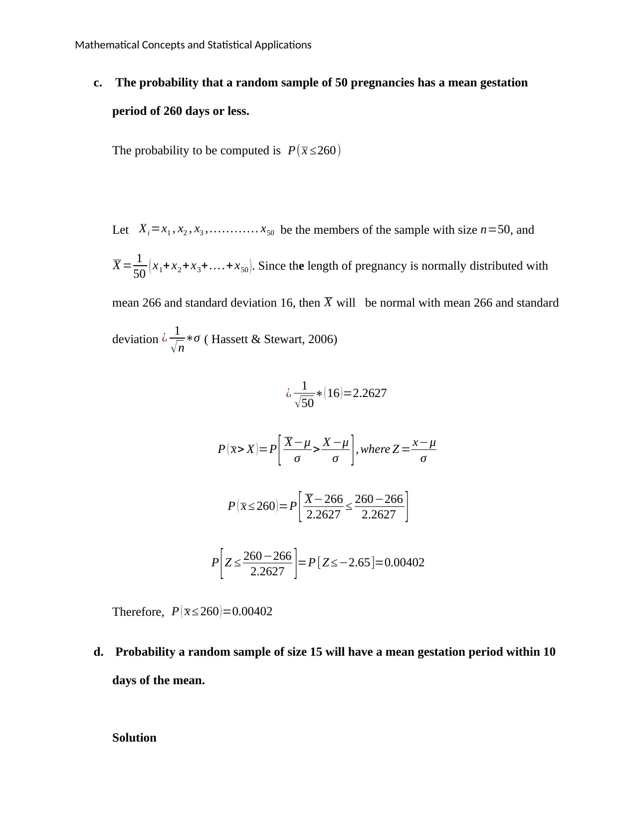
c. The probability that a random sample of 50 pregnancies has a mean gestation
period of 260 days or less.
The probability to be computed is P( x ≤260)
Let Xi =x1 , x2 , x3 , … … … … x50 be the members of the sample with size n=50, and
X = 1
50 ( x1+x2 + x3+ … .+ x50 ). Since the length of pregnancy is normally distributed with
mean 266 and standard deviation 16, then X will be normal with mean 266 and standard
deviation ¿ 1
√n∗σ ( Hassett & Stewart, 2006)
¿ 1
√50∗ ( 16 )=2.2627
P ( x> X ) =P [ X−μ
σ > X −μ
σ ] , where Z = x−μ
σ
P ( x ≤ 260 ) =P [ X−266
2.2627 ≤ 260−266
2.2627 ]
P [ Z ≤ 260−266
2.2627 ]=P [ Z ≤−2.65]=0.00402
Therefore, P ( x ≤ 260 )=0.00402
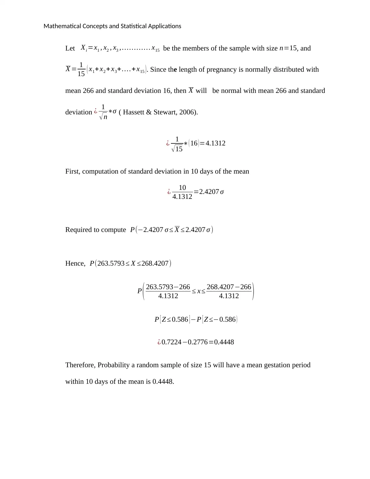
d. Probability a random sample of size 15 will have a mean gestation period within 10
days of the mean.
Solution

Mathematical Concepts and Statistical Applications
Let Xi =x1 , x2 , x3 , … … … … x15 be the members of the sample with size n=15, and
X = 1
15 ( x1+ x2 + x3+… .+x15 ). Since the length of pregnancy is normally distributed with
mean 266 and standard deviation 16, then X will be normal with mean 266 and standard
deviation ¿ 1
√n∗σ ( Hassett & Stewart, 2006).
¿ 1
√ 15∗ ( 16 ) =4.1312
First, computation of standard deviation in 10 days of the mean
¿ 10
4.1312 =2.4207 σ
Required to compute P(−2.4207 σ ≤ X ≤ 2.4207 σ )
Hence, P(263.5793 ≤ X ≤268.4207)
P ( 263.5793−266
4.1312 ≤ x ≤ 268.4207−266
4.1312 )
P [ Z ≤ 0.586 ] −P [ Z ≤−0.586 )
¿ 0.7224−0.2776=0.4448
Therefore, Probability a random sample of size 15 will have a mean gestation period
within 10 days of the mean is 0.4448.

Mathematical Concepts and Statistical Applications
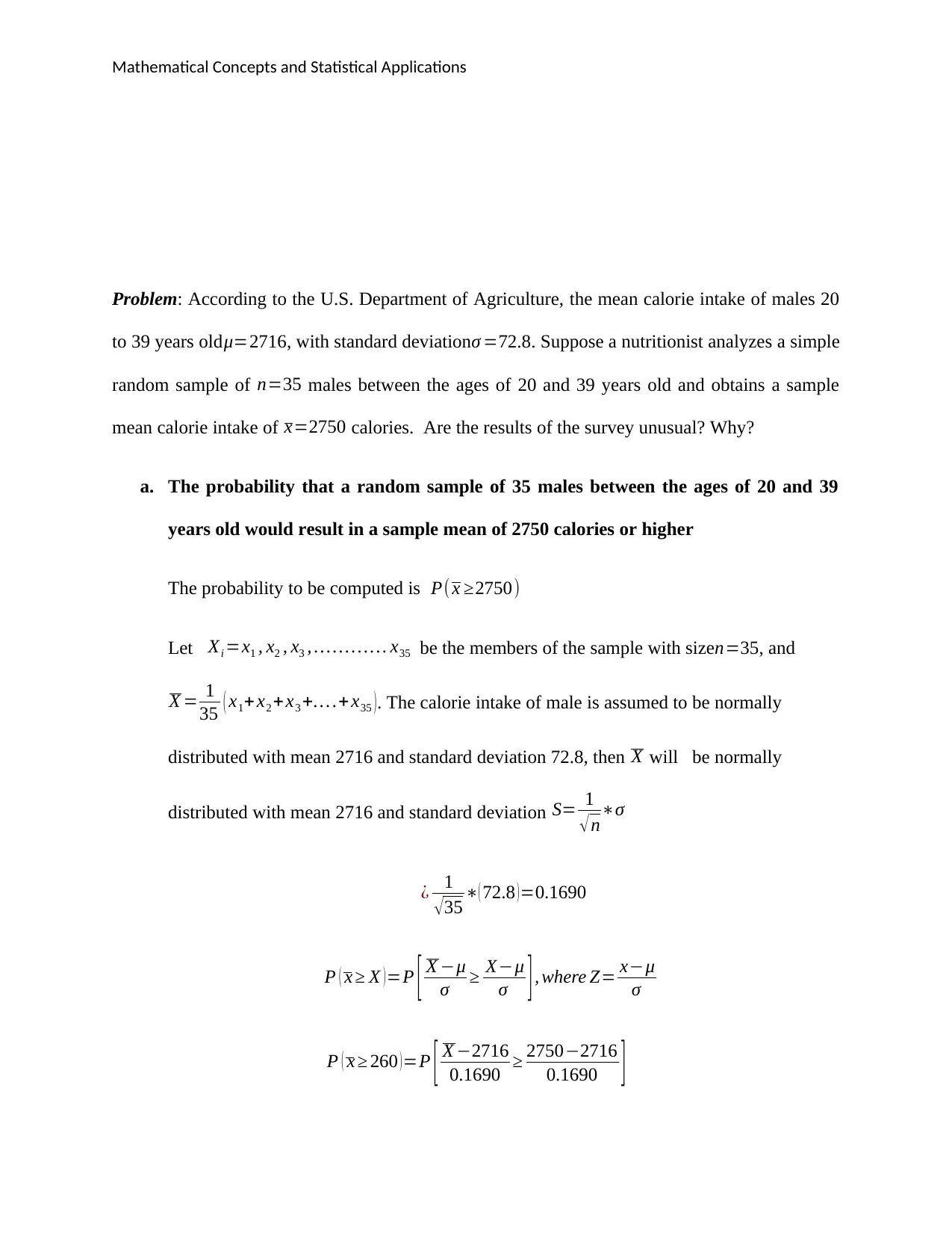
Problem: According to the U.S. Department of Agriculture, the mean calorie intake of males 20
to 39 years old μ=2716, with standard deviationσ =72.8. Suppose a nutritionist analyzes a simple
random sample of n=35 males between the ages of 20 and 39 years old and obtains a sample
mean calorie intake of x=2750 calories. Are the results of the survey unusual? Why?
a. The probability that a random sample of 35 males between the ages of 20 and 39
years old would result in a sample mean of 2750 calories or higher
The probability to be computed is P( x ≥2750)
Let Xi =x1 , x2 , x3 , … … … … x35 be the members of the sample with sizen=35, and
X = 1
35 ( x1+x2 + x3 +… .+ x35 ). The calorie intake of male is assumed to be normally
distributed with mean 2716 and standard deviation 72.8, then X will be normally
distributed with mean 2716 and standard deviation S= 1
√n∗σ
¿ 1
√35 ∗( 72.8 )=0.1690
P ( x ≥ X ) =P [ X −μ
σ ≥ X−μ
σ ] , where Z= x−μ
σ
P ( x ≥ 260 ) =P [ X −2716
0.1690 ≥ 2750−2716
0.1690 ]

Mathematical Concepts and Statistical Applications
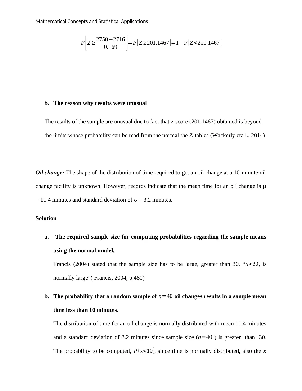
P [Z ≥ 2750−2716
0.169 ]=P [ Z ≥201.1467 ] =1−P [ Z <201.1467 ]
b. The reason why results were unusual
The results of the sample are unusual due to fact that z-score (201.1467) obtained is beyond
the limits whose probability can be read from the normal the Z-tables (Wackerly eta l., 2014)
Oil change: The shape of the distribution of time required to get an oil change at a 10-minute oil
change facility is unknown. However, records indicate that the mean time for an oil change is μ
= 11.4 minutes and standard deviation of σ = 3.2 minutes.
Solution
a. The required sample size for computing probabilities regarding the sample means
using the normal model.
Francis (2004) stated that the sample size has to be large, greater than 30. “n>30, is
normally large”( Francis, 2004, p.480)
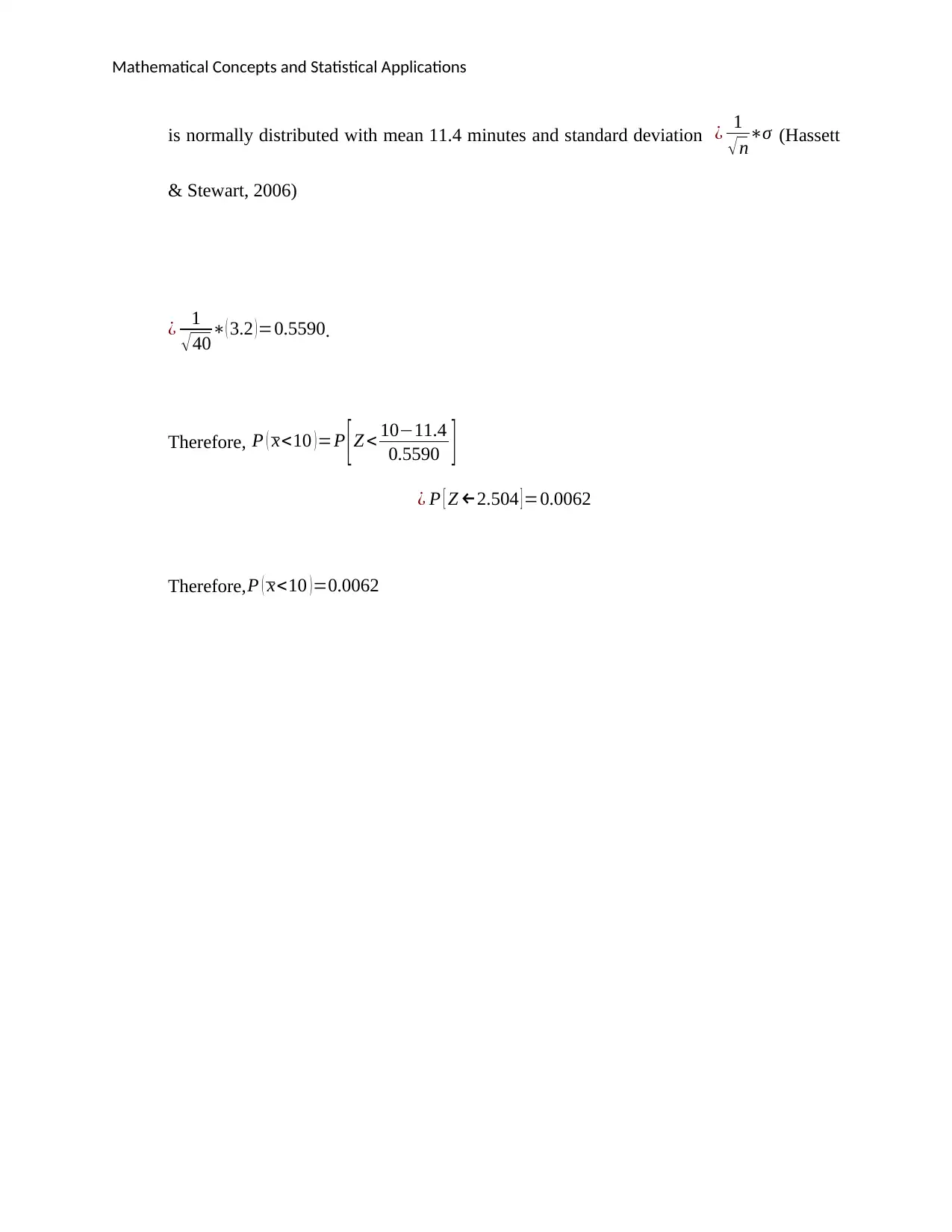
b. The probability that a random sample of n=40 oil changes results in a sample mean
time less than 10 minutes.
The distribution of time for an oil change is normally distributed with mean 11.4 minutes
and a standard deviation of 3.2 minutes since sample size (n=40 ) is greater than 30.
The probability to be computed, P ( x<10 ), since time is normally distributed, also the x

Mathematical Concepts and Statistical Applications
is normally distributed with mean 11.4 minutes and standard deviation ¿ 1
√n∗σ (Hassett
& Stewart, 2006)
¿ 1
√ 40∗( 3.2 ) =0.5590.
Therefore, P ( x<10 )=P [Z < 10−11.4
0.5590 ]
¿ P [ Z ←2.504 ] =0.0062
Therefore, P ( x<10 ) =0.0062

Mathematical Concepts and Statistical Applications
Continued in the next page
Binomial Distributions – Normal Approximation to Binomial Distributions – Sampling
Binomial Distributions
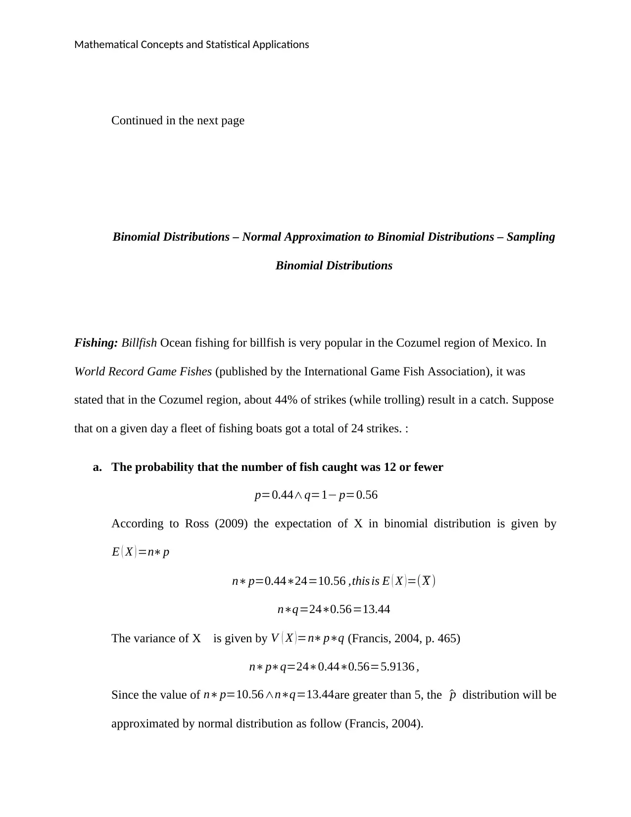
Fishing: Billfish Ocean fishing for billfish is very popular in the Cozumel region of Mexico. In
World Record Game Fishes (published by the International Game Fish Association), it was
stated that in the Cozumel region, about 44% of strikes (while trolling) result in a catch. Suppose
that on a given day a fleet of fishing boats got a total of 24 strikes. :
a. The probability that the number of fish caught was 12 or fewer
p=0.44∧q=1− p=0.56
According to Ross (2009) the expectation of X in binomial distribution is given by
E ( X ) =n∗p
n∗p=0.44∗24=10.56 ,this is E ( X )=(X )
n∗q=24∗0.56=13.44
The variance of X is given by V ( X ) =n∗p∗q (Francis, 2004, p. 465)
n∗p∗q=24∗0.44∗0.56=5.9136 ,
Since the value of n∗p=10.56∧n∗q=13.44are greater than 5, the ^p distribution will be
approximated by normal distribution as follow (Francis, 2004).

Mathematical Concepts and Statistical Applications
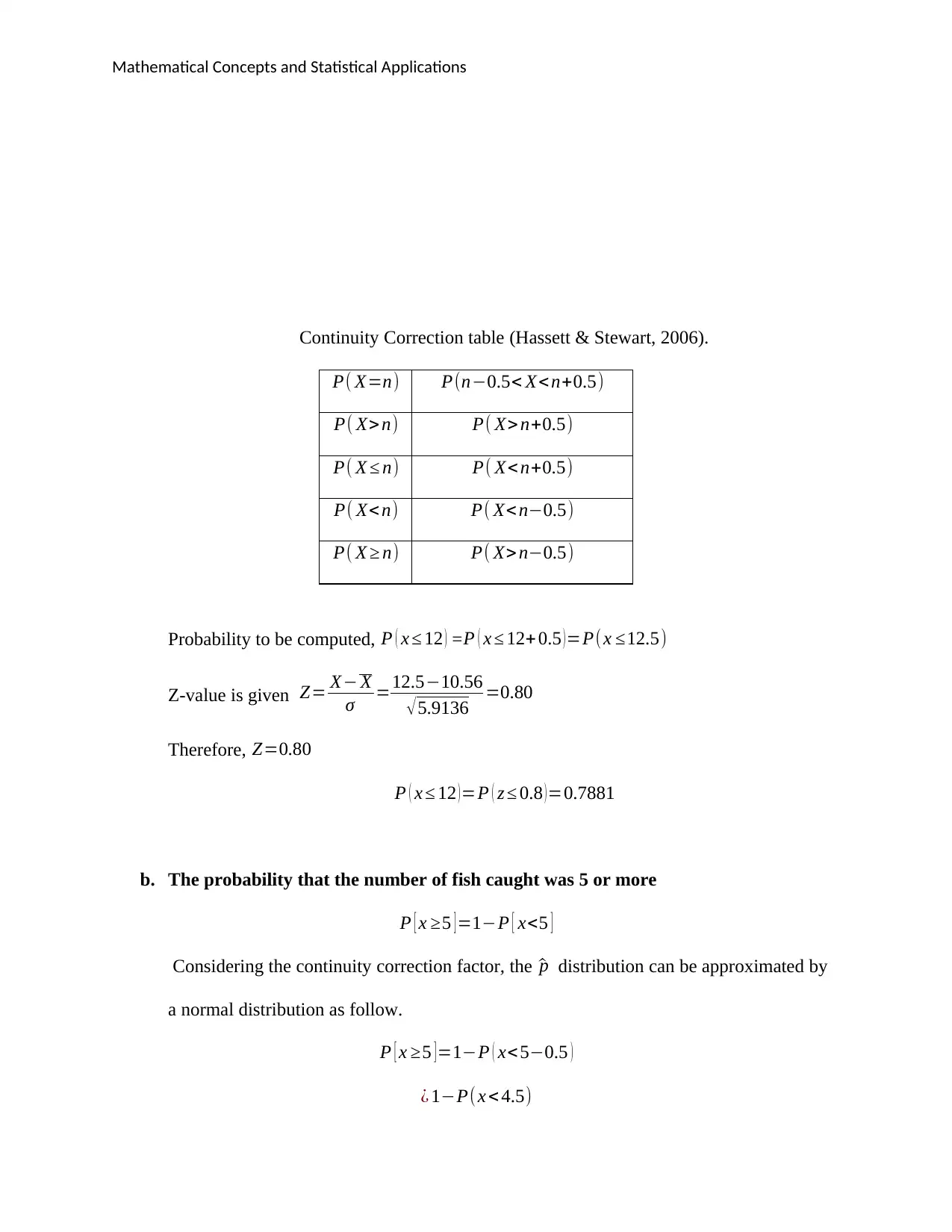
Continuity Correction table (Hassett & Stewart, 2006).
P( X=n) P(n−0.5< X< n+0.5)
P( X> n) P( X> n+0.5)
P( X ≤ n) P( X< n+0.5)
P( X< n) P( X< n−0.5)
P( X ≥ n) P( X> n−0.5)
Probability to be computed, P ( x ≤ 12 ) = P ( x ≤ 12+ 0.5 ) =P(x ≤12.5)
Z-value is given Z= X− X
σ =12.5−10.56
√5.9136 =0.80
Therefore, Z=0.80
P ( x ≤ 12 )=P ( z ≤ 0.8 )=0.7881
b. The probability that the number of fish caught was 5 or more
P [ x ≥5 ] =1−P [ x<5 ]
Considering the continuity correction factor, the ^p distribution can be approximated by
a normal distribution as follow.
P [ x ≥5 ]=1−P ( x<5−0.5 )
¿ 1−P(x < 4.5)

Mathematical Concepts and Statistical Applications
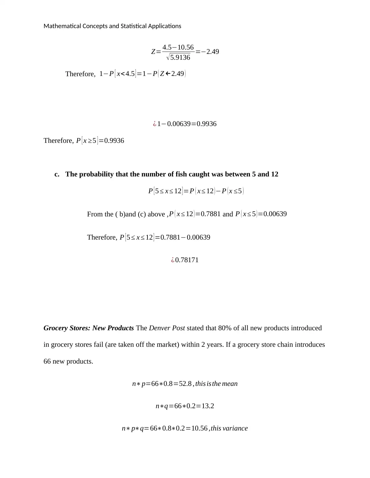
Z= 4.5−10.56
√5.9136 =−2.49
Therefore, 1−P [ x< 4.5 ] =1−P ( Z ←2.49 )
¿ 1−0.00639=0.9936
Therefore, P [ x ≥5 ]=0.9936
c. The probability that the number of fish caught was between 5 and 12
P [ 5 ≤ x ≤ 12 ] =P ( x ≤ 12 ) −P ( x ≤5 )
From the ( b)and (c) above , P ( x ≤ 12 ) =0.7881 and P ( x ≤ 5 ) =0.00639
Therefore, P [ 5 ≤ x ≤ 12 ] =0.7881−0.00639
¿ 0.78171
Grocery Stores: New Products The Denver Post stated that 80% of all new products introduced
in grocery stores fail (are taken off the market) within 2 years. If a grocery store chain introduces
66 new products.
n∗p=66∗0.8=52.8 , this isthe mean
n∗q=66∗0.2=13.2
n∗p∗q=66∗0.8∗0.2=10.56 ,this variance

Mathematical Concepts and Statistical Applications
Therefore, standard deviation ( σ ) =3.25
Since, the values of n∗p=52.8∧n∗q=13.2 are greater than 5 then Continuity Correction factor
will be utilized in approximating this distribution to normal one (Ross, 2006) .
a. The probability that within 2 years 47 or more fail
P ( x ≥ 47 ) =1−P( x < 47)
Considering the continuity correction factor
Z= 46.5−52.8
3.25 =−1.94
Therefore, P ( x ≥ 47 )=1−P ( Z ←1.94 )
¿ 1−0.02619¿ 0.9738
b. The probability that within 2 years 58 or fewer fail
P( x ≤58)
Considering the continuity correction factor, the ^p distribution can be approximated by a
normal distribution ( Ross, 2009).
Z=58.5−52.8
3.25 =1.75
Therefore,
P ( x ≤ 58 ) =P ( Z ≤1.75 ) =0.9599

Mathematical Concepts and Statistical Applications
Thus P ( x ≤ 58 )=0.9599
c. The probability that within 2 years 15 or more succeed
P ( x ≥ 15 ) =1−P ( x< 15)
In this case, the mean be give n∗q=13.2
Considering the continuity correction factor, the ^p distribution can be approximated by a
normal distribution as follow.
Z=14.5−13.2
3.25 =0.4
P ( x ≥ 15 )=1−P ( Z< 0.4 )
¿ 1−0.6554=0.3446
Thus, P ( x ≥ 15 )=0.3446
d. The probability that within 2 years fewer than 10 succeed
In this case, the mean is 13.2
P( x <10)
The ^p distribution can be approximated by normal distribution using continuity
correction factor as follow.
Z= 9.5−13.2
3.25 =−1.14
Therefore, P ( x<10 ) =P ( Z ←1.14 ) =0.1271

Mathematical Concepts and Statistical Applications
Thus, P ( x<10 )=0.1271
Crime: Murder: What are the chances that a person that is murdered actually knew the
murderer? The answer to this question explains why a lot of police detective work begins with
relatives and friends of the victim! About 64% of the people who are murdered actually knew the
person who committed the murder. (Chances: Risk and Odds in Everyday Life by James Burke)
Suppose that a detective file in New Orleans has 63 current unsolved murders. :
p=0.64∧q=0.36
n∗p=63∗0.64=40.32, mean(x)
n∗q=63∗0.36=22.68
n∗p∗q=14.5152 , variance σ 2 , thus standard deviation σ=3.8099
Since the values of n∗p=40.32∧n∗q=22.68 are greater than 5, the ^p distribution can
be approximated by normal distribution using continuity correction factor as follow
(Francis, 2004).
a. The probability that at least 35 of the victims knew their murderers
P ( x ≥ 35 ) =1−P (x< 35)
Considering the continuity correction factor, the ^p distribution can be approximated by a
normal distribution as follow
Z=34.5−40.32
3.8099 =−1.53

Mathematical Concepts and Statistical Applications
Therefore, 1−P ( x <35 )=1−P ( Z ←1.53 )=1−0.06301=0.937
Thus, P ( x ≥ 35 )=0.937
b. The probability that at most 48 of the victims knew their murderers
P( x ≤ 48)
Considering the continuity correction factor, the ^p distribution can be approximated by a
normal distribution as follow
Z= 48.5−40.32
3.8099 =2.15
Therefore, P ( x ≤ 48 ) =P ( Z ≤ 2.15 ) =0.9842
Thus, P ( x ≤ 48 ) =0.9842
Basic Computation: ^p distribution Suppose we have a binomial experiment in which success is
defined to be a particular quality or attribute that interests us.
a. Suppose n=33 and p=0.21. Can we approximate the ^p distribution by a normal
distribution? Why? What are the values of μ ^p andσ ^p
Solution
n∗p=33∗0.21=6.93mean( X)

Mathematical Concepts and Statistical Applications
n∗q=33∗0.79=26.07
n∗p∗q=33∗0.21∗0.79=5.4747 , variance(σ 2
^p )
The ^p distribution can be approximated by normal distribution since the values of
n∗p=6.93 and n∗q=26.07 are greater than 5
The value of μ ^p= X=6.93 and value of σ ^p= √ 5.4747=2.3398
b. Suppose n=25 and p=0.15. Can we safely approximate the ^p distribution by a
normal distribution? Why or why not?
Solution
n∗p=25∗0.15=3.75
n∗q=25∗0.85=21.25
The ^p distribution cannot be safely approximated by normal distribution since the value
of n∗p=3.75 is not greater than 5 even though the value of n∗q=21.25 is greater than
5. At the same time, sample size n=25 is less than 30(Francis 2004, p. 480).
c. Suppose n=48 and p=0.15. Can we approximate the ^p distribution by a normal
distribution? Why? What are the values of μ ^p and σ ^p?
Solution
n∗p=48∗0.15=7.2 , mean( X )
n∗q=48∗0.85=40.8

Mathematical Concepts and Statistical Applications
n∗p∗q=48∗0.15∗0.85=6.12 , Variance(σ2
^p )
Since the value of n∗p=7.2∧n∗q=40.8 are greater than 5, ^p distribution can be safely
approximated by a normal distribution (Ross, 2009).
The values of μ ^p= X=7.2 and σ ^p= √ 6.12=2.4739
Basic Computation: ^p distribution Suppose we have a binomial experiment in which success is
defined to be a particular quality or attribute that interests us.
a. Suppose n=100 and p=0.23. Can we approximate the ^p distribution by a normal
distribution? Why? What are the values of μ ^p and σ ^p.
Solution
n∗p=100∗0.23=23 ,mean X
n∗p=100∗0.77=77
n∗p∗q=100∗0.23∗0.77=17.71, variance σ2
^p
The ^p distribution can be approximated by normal distribution since the values of
n∗p=23 and n∗q=77 are greater than 5(Francis 2004).
The values of μ ^p= X=23 and σ ^p= √17.71=4.2083

Mathematical Concepts and Statistical Applications
b. Suppose n=20 and p=0.23. Can we safely approximate the ^p distribution by a
normal distribution? Why or why not?
Solution
The expectation of X in binomial distribution is given by E ( X ) =n∗p (Ross, 2009,
p.139)
n∗p=20∗0.23=4.6 , mean X
n∗p=20∗0.77=15.4
n∗p∗q=20∗0.23∗0.77=3.542 , variance σ2
^p
The ^p distribution cannot be safely approximated by normal distribution since the value
of n∗p=4.6is not greater than 5. Even though the value of n∗q=15.4 is greater than 5,
the sample size n=20 is also less than 30.

Mathematical Concepts and Statistical Applications
Reference
1. Francis, A. (2004). Business mathematics and statistics. Cengage Learning
EMEA.
2. Hassett, M. J., & Stewart, D. (2006). Probability for risk management.
Actex Publications.
3. Ross, S. (2009). A First Course in Probability 8th Edition. Pearson.
4. Wackerly, D., Mendenhall, W., & Scheaffer, R. L. (2014). Mathematical
statistics with applications. Cengage Learning.