Mathematics for Construction: Detailed Solutions for Tasks 2, 3, & 4

This document presents a comprehensive solution to a construction mathematics assignment, addressing various tasks and scenarios. Task 2 focuses on statistical analysis, including creating histograms, determining the mode, calculating cumulative frequency distributions, and finding mean, range, and standard deviation for revenue data. Task 3 delves into wave analysis, calculating phase, amplitude, frequency, and displacement, using compound angle formulas, and plotting wave functions. Task 4 explores normal distribution, hypothesis testing, and vector geometry, including determining allowable intervals for bulb replacement, performing hypothesis testing using one-tailed and two-tailed tests, and calculating distances and angles between vectors. The assignment also includes practical considerations, such as the impact of replacement time and cost for different types of bulbs. The solutions are detailed and provide step-by-step explanations, making it a valuable resource for students studying mathematics for construction.

8 Mathematics for
Construction

Table of Contents
TASK 2 ...........................................................................................................................................3
Scenario 1.....................................................................................................................................3
Scenario 2.....................................................................................................................................6
TASK 3..........................................................................................................................................12
Scenario 1...................................................................................................................................12
Scenario 2...................................................................................................................................16
TASK 4..........................................................................................................................................18
Scenario 1...................................................................................................................................18
Scenario 2 ..................................................................................................................................20
Scenario 3...................................................................................................................................22

TASK 2
Scenario 1
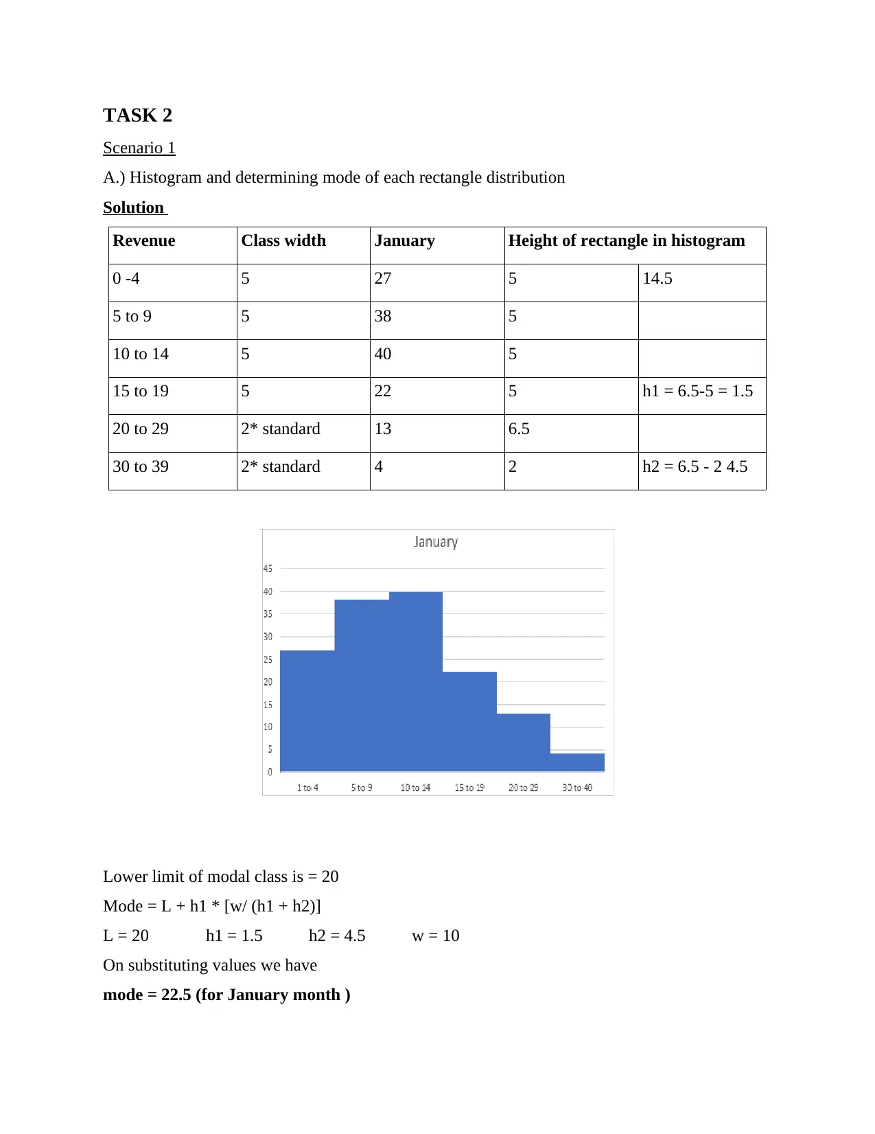
A.) Histogram and determining mode of each rectangle distribution
Solution
Revenue Class width January Height of rectangle in histogram
0 -4 5 27 5 14.5
5 to 9 5 38 5
10 to 14 5 40 5
15 to 19 5 22 5 h1 = 6.5-5 = 1.5
20 to 29 2* standard 13 6.5
30 to 39 2* standard 4 2 h2 = 6.5 - 2 4.5
Lower limit of modal class is = 20
Mode = L + h1 * [w/ (h1 + h2)]
L = 20 h1 = 1.5 h2 = 4.5 w = 10
On substituting values we have
mode = 22.5 (for January month )

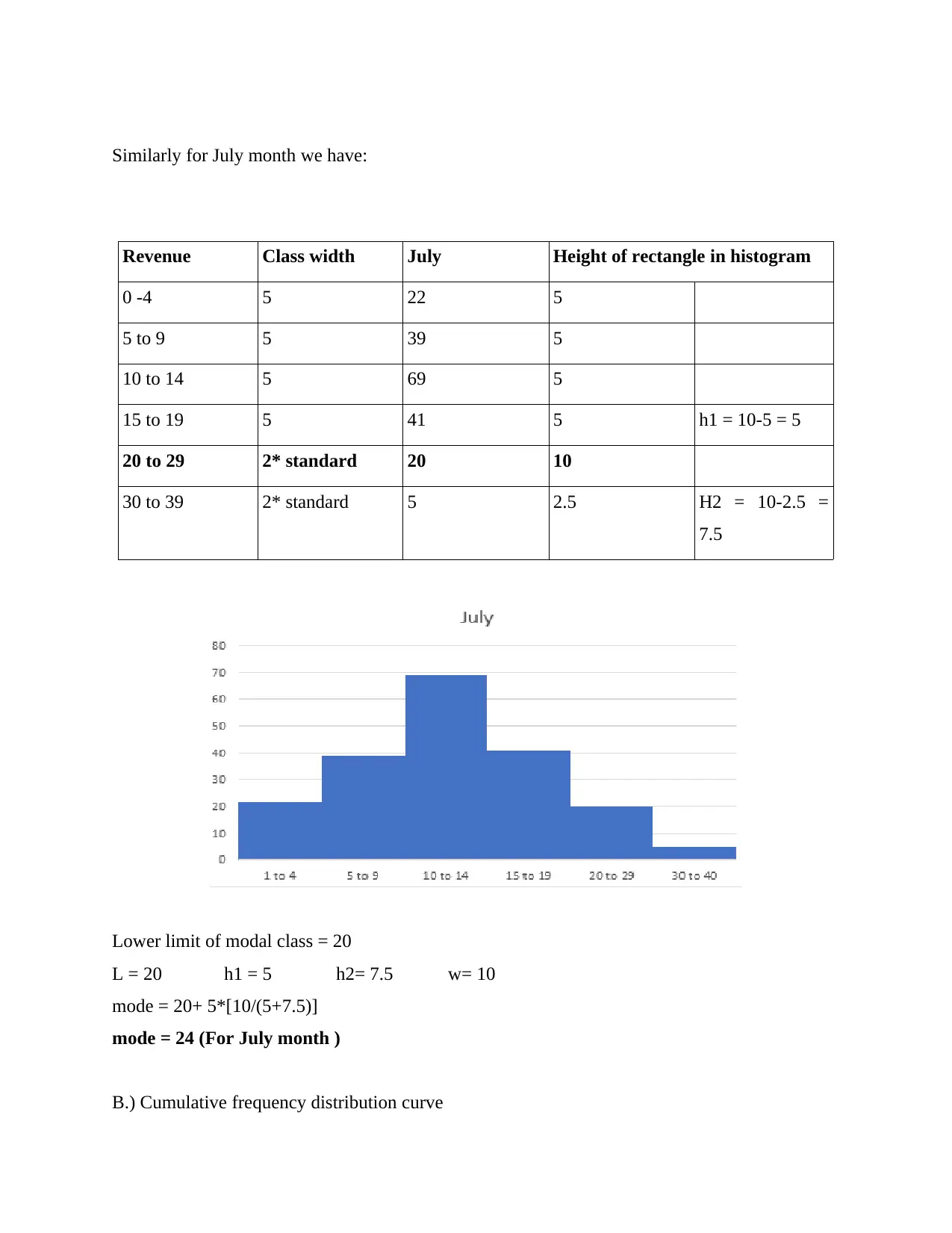
Similarly for July month we have:
Revenue Class width July Height of rectangle in histogram
0 -4 5 22 5
5 to 9 5 39 5
10 to 14 5 69 5
15 to 19 5 41 5 h1 = 10-5 = 5
20 to 29 2* standard 20 10
30 to 39 2* standard 5 2.5 H2 = 10-2.5 =
7.5
Lower limit of modal class = 20
L = 20 h1 = 5 h2= 7.5 w= 10
mode = 20+ 5*[10/(5+7.5)]
mode = 24 (For July month )
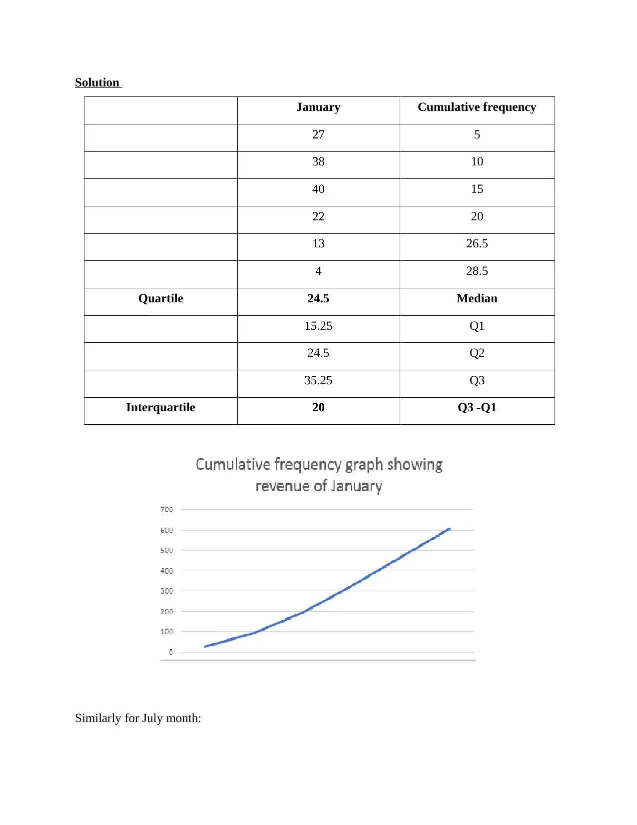
B.) Cumulative frequency distribution curve

Solution
January Cumulative frequency
27 5
38 10
40 15
22 20
13 26.5
4 28.5
Quartile 24.5 Median
15.25 Q1
24.5 Q2
35.25 Q3
Interquartile 20 Q3 -Q1
Similarly for July month:

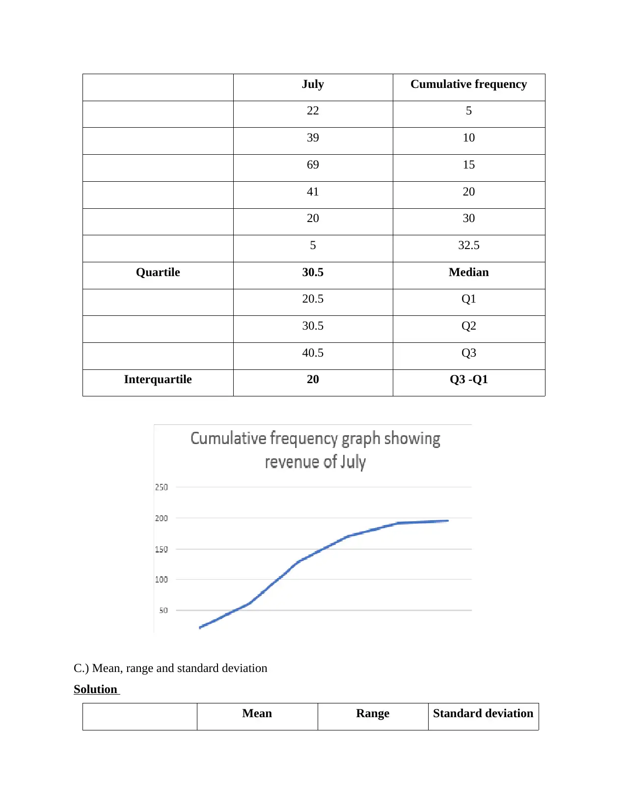
July Cumulative frequency
22 5
39 10
69 15
41 20
20 30
5 32.5
Quartile 30.5 Median
20.5 Q1
30.5 Q2
40.5 Q3
Interquartile 20 Q3 -Q1
C.) Mean, range and standard deviation
Solution
Mean Range Standard deviation

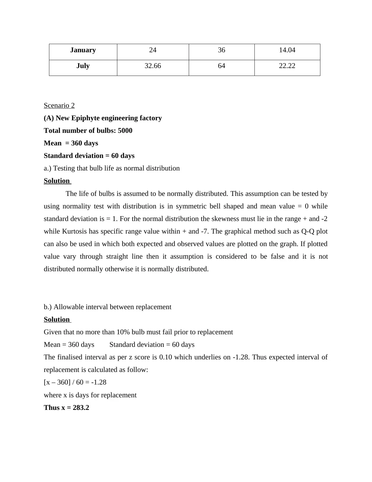
January 24 36 14.04
July 32.66 64 22.22
Scenario 2
(A) New Epiphyte engineering factory
Total number of bulbs: 5000
Mean = 360 days
Standard deviation = 60 days
a.) Testing that bulb life as normal distribution
Solution
The life of bulbs is assumed to be normally distributed. This assumption can be tested by
using normality test with distribution is in symmetric bell shaped and mean value = 0 while
standard deviation is = 1. For the normal distribution the skewness must lie in the range + and -2
while Kurtosis has specific range value within + and -7. The graphical method such as Q-Q plot
can also be used in which both expected and observed values are plotted on the graph. If plotted
value vary through straight line then it assumption is considered to be false and it is not
distributed normally otherwise it is normally distributed.
b.) Allowable interval between replacement
Solution
Given that no more than 10% bulb must fail prior to replacement
Mean = 360 days Standard deviation = 60 days
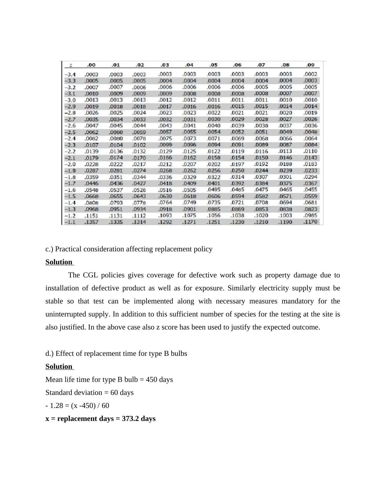
The finalised interval as per z score is 0.10 which underlies on -1.28. Thus expected interval of
replacement is calculated as follow:
[x – 360] / 60 = -1.28
where x is days for replacement
Thus x = 283.2

c.) Practical consideration affecting replacement policy
Solution
The CGL policies gives coverage for defective work such as property damage due to
installation of defective product as well as for exposure. Similarly electricity supply must be
stable so that test can be implemented along with necessary measures mandatory for the
uninterrupted supply. In addition to this sufficient number of species for the testing at the site is
also justified. In the above case also z score has been used to justify the expected outcome.
d.) Effect of replacement time for type B bulbs
Solution
Mean life time for type B bulb = 450 days
Standard deviation = 60 days
- 1.28 = (x -450) / 60
x = replacement days = 373.2 days

e.) Preference for type B bulb in comparison to existing type A bulb
Solution
Despite 25% increment in the cost of bulb type A, the replacement time comparison for
both bulb A and B is provided as below:
Type A (360 days) = 283 days
Type b (450 days) = 373.2 days
Impact = 31.87%
Thus 25% cost increment is not preferable as it is already increasing by 31 days so replacement
must be at average of 360 days and standard deviation of 60 days with less than 10%
f.) Replacement time for type C bulb
Solution
Mean = 432 days
Standard deviation = 45 days
-1.28 = (x- 432) / 45
x = 489.60 days
Thus
Type C Type A Impact
489.6 283 73.00%
Thus among all choices of bulb for New Epiphyte engineering with total 5000 bulbs type C is
most preferred because its standard deviation is declining. The percentage change of 73%
indicates its higher suitability for adaptation.
B.) Hypothesis testing at % significance level using two tailed and one tailed test
Solution
Sample population = n = 10
Mean age = 27
Variance = 20

Significance level = 0.5
Assumptions:
 Simple random sample
 Normally distributed population
Hypothesis
H0: = 30
H1: is not equal to 30
Test statistic
Variance is known so implication of z test statistic:
Test statistic distribution:
If assumptions are true then H0 is true and then test statistic follow standard normal
distribution. Thus hypothesis testing and z score calculation are as follows:
Decision rule :
z value underlying in rejection zone is reject null hypothesis while failure to reject null
hypothesis if it underlies in non-rejection zone.
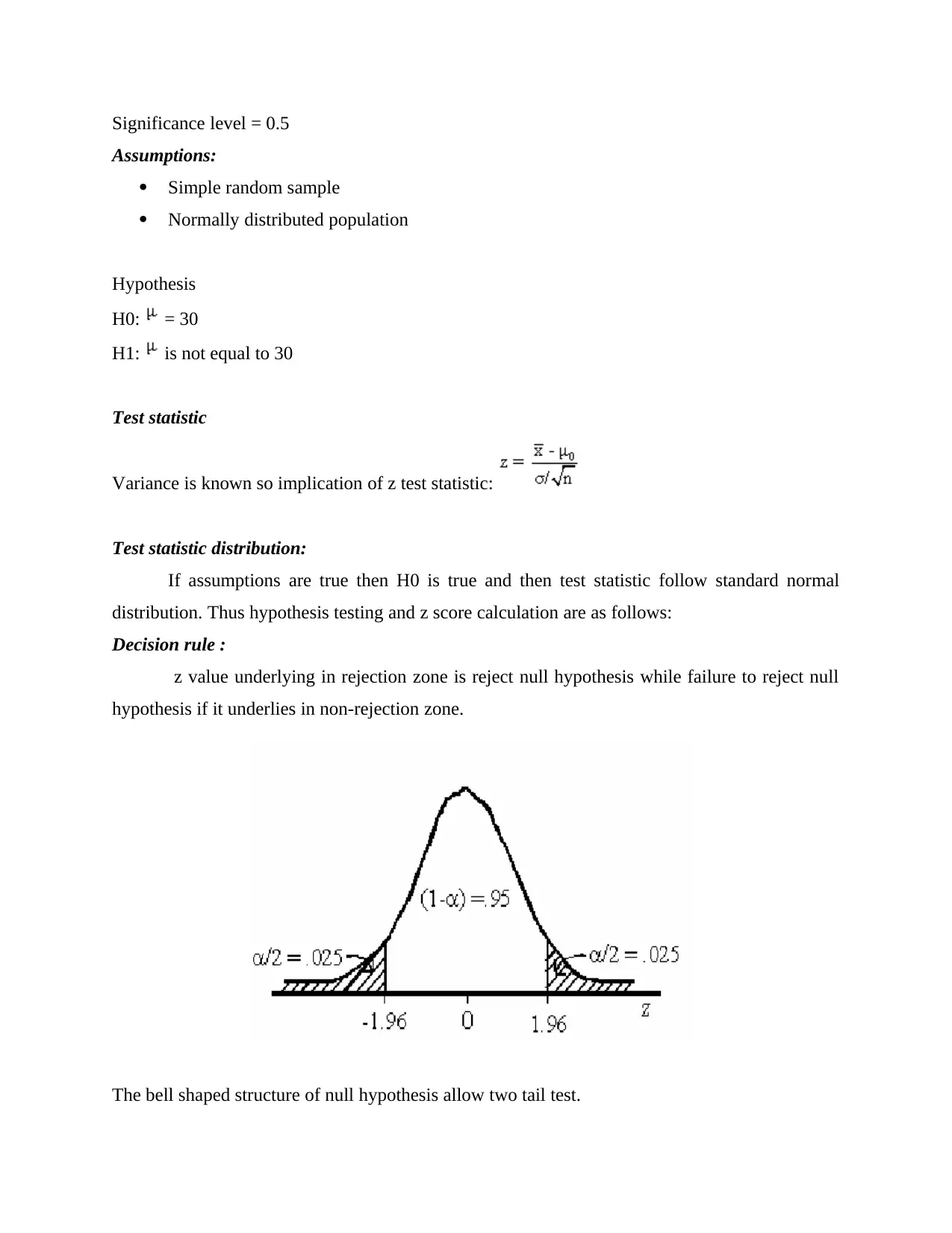
The bell shaped structure of null hypothesis allow two tail test.

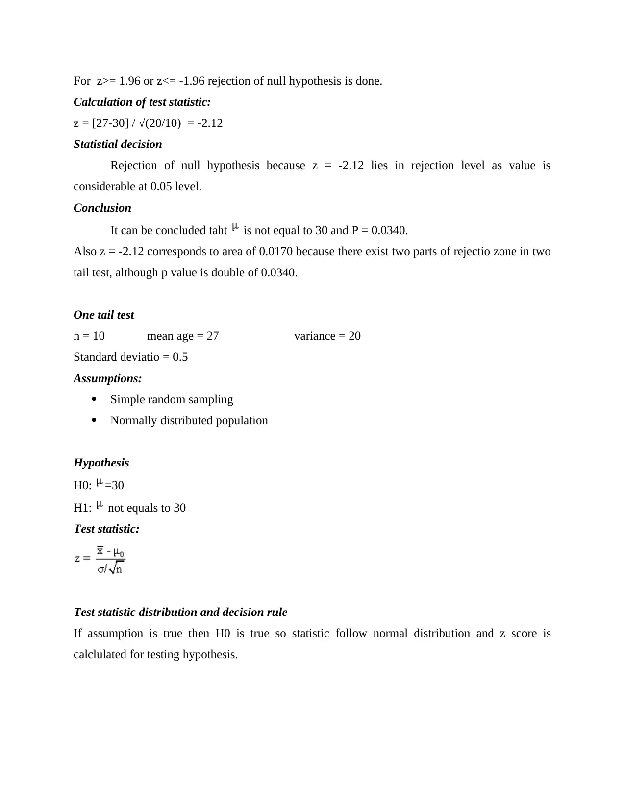
For z>= 1.96 or z<= -1.96 rejection of null hypothesis is done.
Calculation of test statistic:
z = [27-30] / √(20/10) = -2.12
Statistial decision
Rejection of null hypothesis because z = -2.12 lies in rejection level as value is
considerable at 0.05 level.
Conclusion
It can be concluded taht is not equal to 30 and P = 0.0340.
Also z = -2.12 corresponds to area of 0.0170 because there exist two parts of rejectio zone in two
tail test, although p value is double of 0.0340.
One tail test
n = 10 mean age = 27 variance = 20
Standard deviatio = 0.5
Assumptions:
 Simple random sampling
 Normally distributed population
Hypothesis
H0: =30
H1: not equals to 30
Test statistic:
Test statistic distribution and decision rule
If assumption is true then H0 is true so statistic follow normal distribution and z score is
calclulated for testing hypothesis.

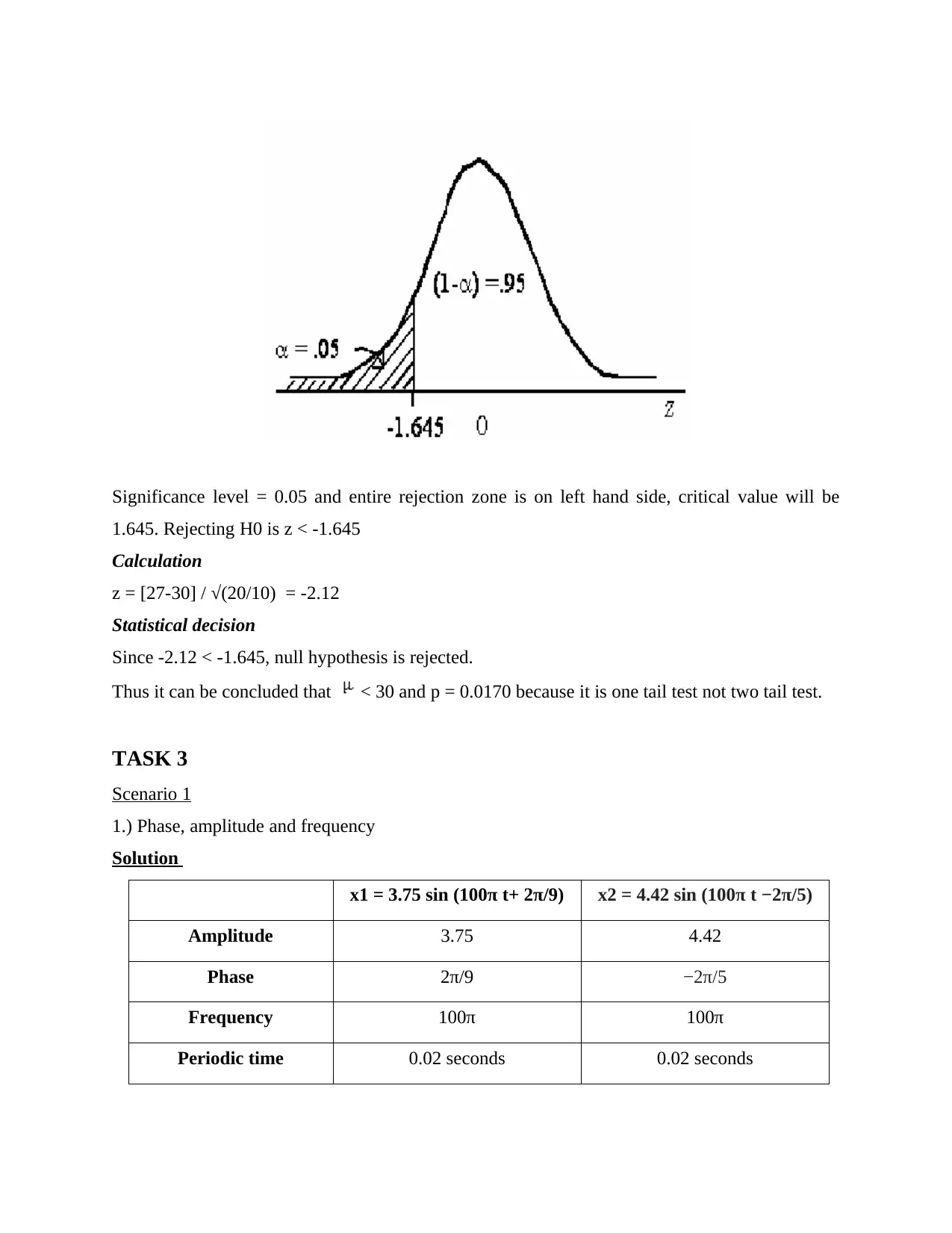
Significance level = 0.05 and entire rejection zone is on left hand side, critical value will be
1.645. Rejecting H0 is z < -1.645
Calculation
z = [27-30] / √(20/10) = -2.12
Statistical decision
Since -2.12 < -1.645, null hypothesis is rejected.
Thus it can be concluded that < 30 and p = 0.0170 because it is one tail test not two tail test.
TASK 3
Scenario 1
1.) Phase, amplitude and frequency
Solution
x1 = 3.75 sin (100π t+ 2π/9) x2 = 4.42 sin (100π t −2π/5)
Amplitude 3.75 4.42
Phase 2π/9 −2π/5
Frequency 100π 100π
Periodic time 0.02 seconds 0.02 seconds