HNCB 8 Mathematics for Construction Assignment Solution - Analysis

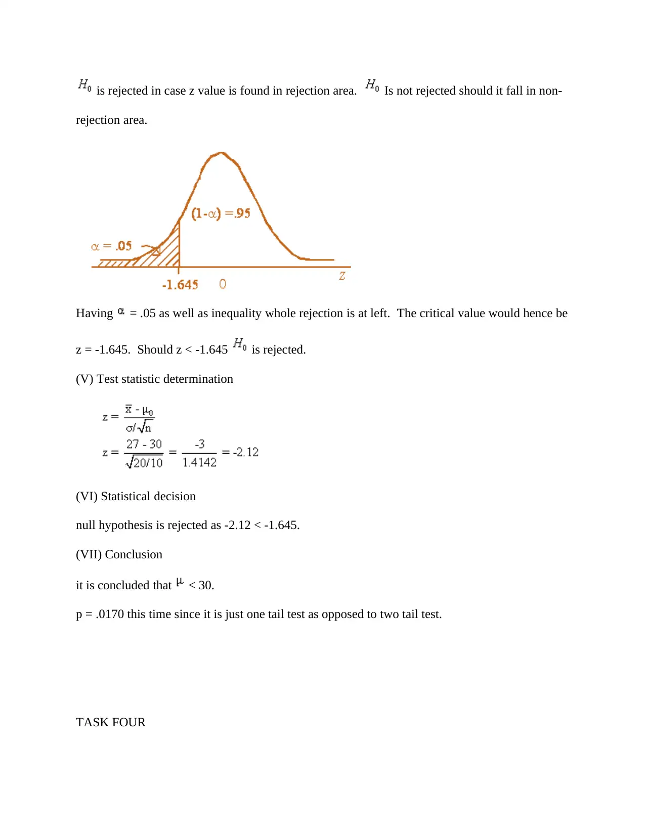
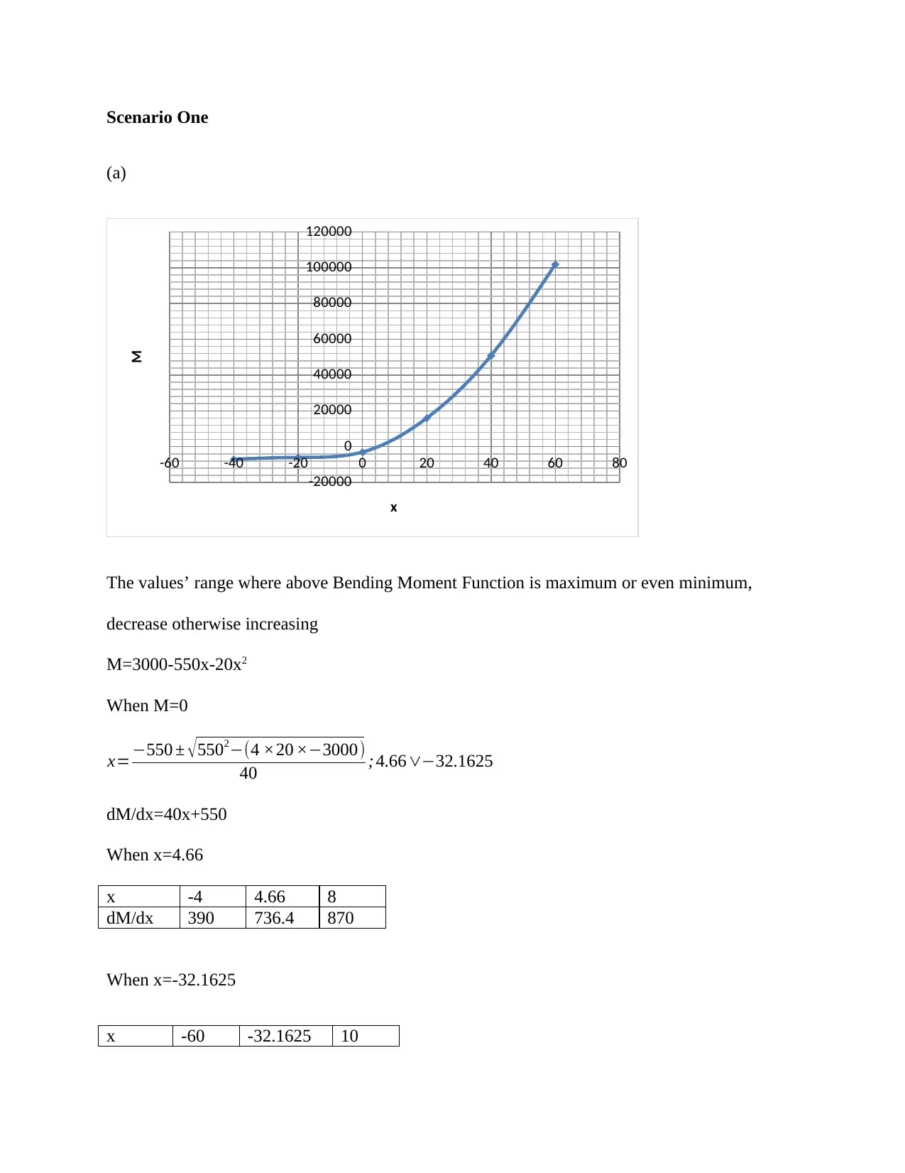
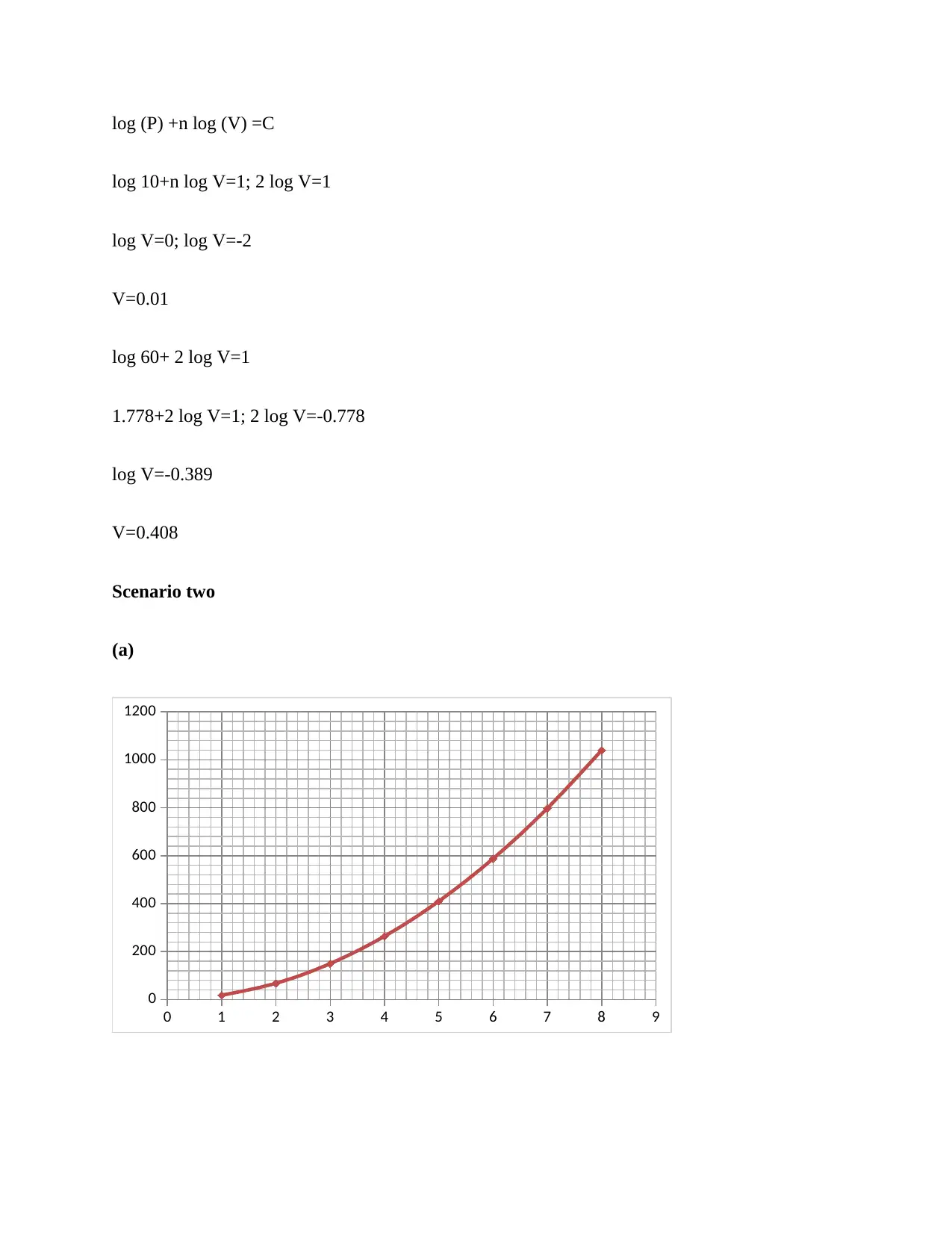
This document presents a comprehensive solution to a Mathematics for Construction assignment, likely for an HNCB 8 course. The assignment covers a range of mathematical concepts and their applications within a construction context. Task 1 involves solving equations related to area and arith...Read More

HNCB 8 MATHEMATICS FOR CONSTRUCTION
By Name
Course
Instructor
Institution
Location
Date

Task 1
Scenario 1
A=26.5; L=w+3.2; w=w
A=LW
w ( w+3.2 ) =26.5
w=−3.2 ± √3.22−4 ×1 ×−26.5
2
¿ 3.2 ± √ 116.24
2
w=3.79 m
L=3.79+3.2=6.99 m
a+ (n-1) d
a+ (5-1)d=4250
a+ (12-1)d=2120
d=304
Daily forfeit=£304
a+4d=4250
d=304
a=4250-(4*304)
a=£3032

Task TWO
Scenario One
0-4 5-9 10-14 15-19 20-29 30-39
0
5
10
15
20
25
30
35
40
45
0 2 4 6 8 10 12
0
50
100
150
200
250
Revenue
Customers

0-4 5-9 10-14 15-19 20-29 30-39
0
10
20
30
40
50
60
70
80
0 2 4 6 8 10 12
0
2
4
6
8
10
12
Revenue
Customers
(c)
Mean=∑ fx/ ∑ f
=1630.5/144=11.323
Range=5 for initial 4 groups and 1o for last two groups
Variance σ2 = ∑ fx2
∑ f −x2
= (26652.25/144)-11.3232

56.875
δ=7.54
Scenario two
Kolmogorov-Smirnov (K-S) & Shapiro-Wilk (S-W) tests may be used in testing of assumption
data sample are extracted from normally distributed population.
The probabilities provided in problem tend to be cumulative meaning till 1st week, 2nd week
Individual probabilities will be 0.10 in week 1, 0.15 (0.25-0.10) in week two1
Individual Failures/week = Total Quantity / Mean Life = 1000 / 3.45 = 289.9
Individual Replacement Cost = (Individual Failures @ week) x (Individual cost of replacement)
= 289.90 x 3.0 = Rs. 869.60
In week 1: 10 % (0.10) of bulbs would fail out of 1000 bulbs meaning 100
In week 2: 15% of bulbs would fail out of 1000 bulbs i.e. 150. Still, 10% of 100 replaced in
week 1 i.e. 10 CUMULATIVE bulbs failed by end of week 2 = 160 (150+10)
Thus, replacing all bulbs at same time at fixed interval as well as substituting individual bulbs
which fail in between would turn out to economical by week 4 end.
[N/B: "Yes we can, if..." One of the ways of aiding in obtaining solution to a [problem of such
type is to respond in affirmative "Yes we can, if..." For this scenario, interrogative is, "Can a
conclusion be made that population mean age is not 30?" Answer, "Yes we can, should it be
possible to eject null hypothesis indicating that it’s 30." Giving response to challenges in similar
manner all times would cause less confusion as well as limited errors.
(I) Data
n = 10 = 20
1 Bauer, , Jörg, Johannes and Detlef. "Impact factors on the cost calculation for building services within the built
environment." Procedia Engineering 171 (2017): 294-301

= 27 = .05
(II) Assumptions
 Sample that is simple and random
 A population that is normally distributed
(III) Hypotheses
: = 30
: 30
(IV) Test statistic
as variance of population is known, z is used as test statistic.
(a) Test statistic distribution
should the assumptions be correct as well as true, test statistic conforms to standard normal
distribution. Hence, z score is estimated hence used to test hypothesis2.
(b) Decision rule
is rejected should z value be found in rejection area. Is not rejected should it fall in non-
rejection region.
2 Dreuw, Andreas, and Michael. "The algebraic diagrammatic construction scheme for the polarization propagator
for the calculation of excited states." Wiley Interdisciplinary Reviews: Computational Molecular Science 5, no. 1
(2015): 82-95

Owing to structure of it stands to be a two tail test. Hence, reject if z -1.96 or z
1.96.
(V) Determination of test statistic
(VI) Statistical decision
null hypothesis is rejected since z = -2.12 that is in rejection position. The value is treated to be
significant at .05 level.
(VII) Conclusion
it is concluded that is not 30.
p = .0340
A z value of -2.12 is in correspondence to region of .0170. As there exist two sections to
rejection area in two tail test, value of p is double such that is .0340.
A problem as this may also be attended to via use of confidence interval3. A confidence interval
would be indicative determined z value does not appear interval boundaries. It does not however
provide probability.
3 Mendoza, Francisco, Joan and Antonio. "Application of inert wastes in the construction, operation and closure of
landfills: Calculation tool." Waste management 59 (2017): 276-285

Confidence interval
Similar illustration as one tailed test
(I) Data
n = 10 = 20
= 27 = .05
(II) Assumptions
 simple random sample
 normally distributed population
(III) Hypotheses
: = 30
: 30
(IV) Test statistic
as variance of population is known, z is used as test statistic.
(a) Test statistic distribution
supposes assumptions are right as well as true; test statistic conforms to standard normal
distribution. Hence, a z score is calculated thus used to test hypothesis.
(b) Decision rule

is rejected in case z value is found in rejection area. Is not rejected should it fall in non-
rejection area.
Having = .05 as well as inequality whole rejection is at left. The critical value would hence be
z = -1.645. Should z < -1.645 is rejected.
(V) Test statistic determination
(VI) Statistical decision
null hypothesis is rejected as -2.12 < -1.645.
(VII) Conclusion
it is concluded that < 30.
p = .0170 this time since it is just one tail test as opposed to two tail test.
TASK FOUR

Scenario One
(a)
-60 -40 -20 0 20 40 60 80
-20000
0
20000
40000
60000
80000
100000
120000
x
M
The values’ range where above Bending Moment Function is maximum or even minimum,
decrease otherwise increasing
M=3000-550x-20x2
When M=0
x=−550 ± √ 5502−(4 ×20 ×−3000)
40 ; 4.66∨−32.1625
dM/dx=40x+550
When x=4.66
x -4 4.66 8
dM/dx 390 736.4 870
When x=-32.1625
x -60 -32.1625 10

dM/dx -1850 -736.5 950
As per calculations, function is decreasing
The temperature, Ɵ (⁰C) at time t (mins) of body is given by
Ɵ=300 +100e-0.1t
Evaluate Ɵ for t=0, 1, 2 and 5
Ɵ=300 +100e-0.1(0) =400
Ɵ=300 +100e-0.1(1) =390.48
Ɵ=300 +100e-0.1(2) =381.87
Ɵ=300 +100e-0.1(5) =360.65
Range of temperature for positive t= (360.65 to 400)
(c) 0=300 +100e-0.1t
100e-0.1t=-300; e-0.1t=-3
0.9048t=-3; t=-3.3
log (P) +n log (V)-log C
Log (P) + log (V) n=log C
P.Vn=C; hence
PVn=C
log (P) +n log (V)-log C

log (P) +n log (V) =C
log 10+n log V=1; 2 log V=1
log V=0; log V=-2
V=0.01
log 60+ 2 log V=1
1.778+2 log V=1; 2 log V=-0.778
log V=-0.389
V=0.408
Scenario two
(a)
0 1 2 3 4 5 6 7 8 9
0
200
400
600
800
1000
1200

(b) Calculus is usable in calculation of time for maximum as well as minimum production
alongside time where no production will occur. Maximum production takes place when C is
maximum which is reverse for the case of minimum production. Still calculus may be used
determination production amount at different production time thus enabling production trend
prediction.
(c) C=16t-2+2t-
0=16t-2+2t-; 16t-2+2t-=0
16t-2=-2t-
t-1=-1/8; t=-8
(d) dC/dt=32t-3-2t-2
t -20 -8 4
dC/dt -0.009 -0.09375 0.375
dC/dt =32t-3-2t-2
32(-20)-3-2(-20)-2=-0.004-0.005
=-0.009
dC/dt=32t-3-2t-2
32(-8)-3-2(-8)-2=-0.0625-0.03125
=-0.09375
dC/dt=32t-3-2t-2
32(4)-3-2(4)-2=0.5-0.125

=-0.375
There is no further minimum production cost as graph turns just at a single point that is 8
seconds. This will remain the minimum production time hence miniumum cost of production.
Scenario Three
-25 -20 -15 -10 -5 0 5 10 15 20 25
0
500000
1000000
1500000
2000000
2500000
3000000
3500000
E3t
t

References
B. Bauer, K. Jörg, W. Johannes and H. Detlef. "Impact factors on the cost calculation for
building services within the built environment." Procedia Engineering 171 (2017): 294-301.
A. Dreuw and W. Michael. "The algebraic diagrammatic construction scheme for the
polarization propagator for the calculation of excited states." Wiley Interdisciplinary Reviews:
Computational Molecular Science 5, no. 1 (2015): 82-95
Mendoza, J.C. Francisco, E.A. Joan and G. I. Antonio. "Application of inert wastes in the
construction, operation and closure of landfills: Calculation tool." Waste management 59 (2017):
276-285