Applications of Mathematical Methods in Mechanical Engineering

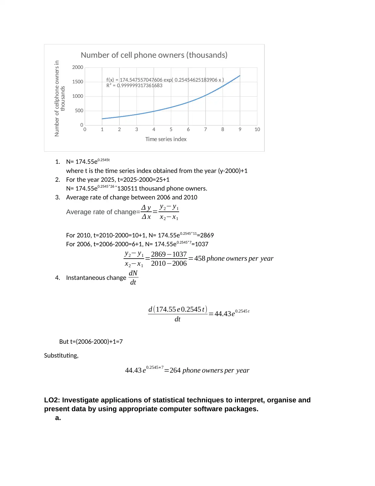
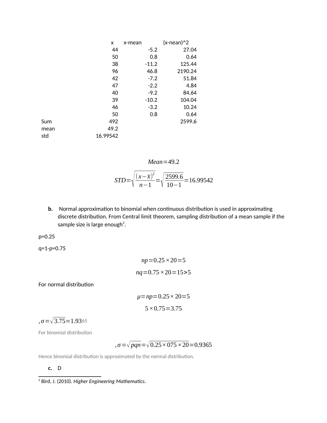
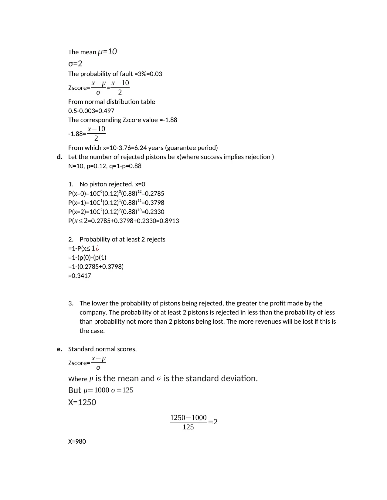
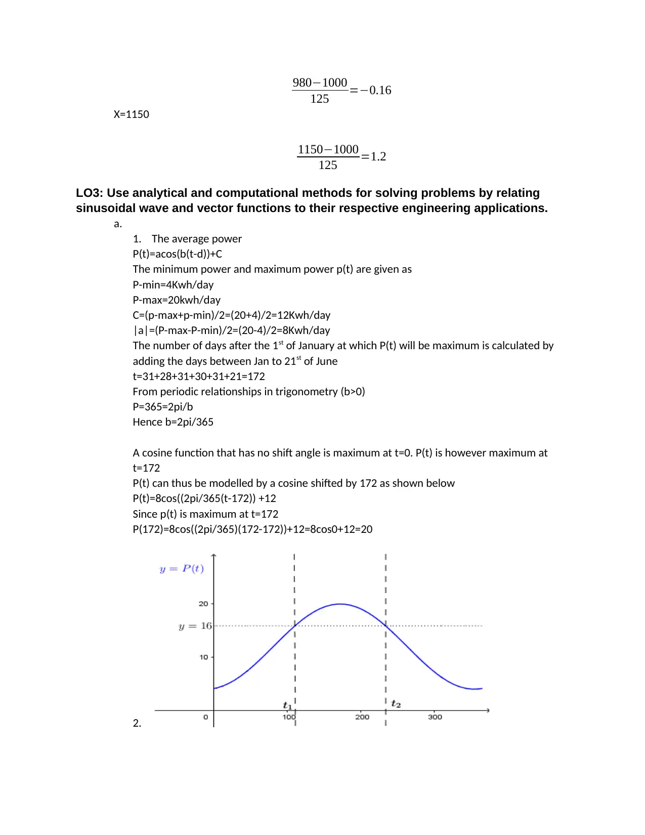
This document presents a comprehensive solution to an engineering mathematics assignment, covering a wide range of topics relevant to mechanical engineering. The assignment addresses multiple learning outcomes, including the identification of mathematical methods in engineering examples, the investigation of statistical techniques for data interpretation, and the application of analytical and computational methods to solve problems involving sinusoidal waves and vector functions. Furthermore, it explores the use of differential and integral calculus in solving engineering problems. The solution includes detailed calculations, graphical representations, and explanations, providing a thorough understanding of the concepts. The document also references several academic sources and includes solutions to problems involving dimensional analysis, series, time-speed relations, radioactivity, time series analysis, statistical analysis, binomial distribution, normal distribution, and applications of calculus. The assignment showcases the practical application of mathematical principles in various engineering scenarios.

Table of Contents
LO1: Identify the relevance of mathematical methods to a variety of conceptualized
engineering examples...........................................................................................................................2
LO2: Investigate applications of statistical techniques to interpret, organise and present
data by using appropriate computer software packages.............................................................5
LO3: Use analytical and computational methods for solving problems by relating
sinusoidal wave and vector functions to their respective engineering applications............8
LO4: Examine how differential and integral calculus can be used to solve engineering
problems.................................................................................................................................................11

LO1: Identify the relevance of mathematical methods to a variety of conceptualized
engineering examples.
a. Equating the dimensions of both sides of the equation, we obtain,
Comparing the two sides of the equations, we get
From the third equation, x=0.5, substituting in the second equation, we get y=-0.5 and making
the two substitutions in equation 1, we get z=0
From the values
b. Let
F α ra
F α vb
F α nc
Alternatively
F α ra vb nc
F =k ra rb rc
Where k is a proportionality constant1
[M1L1T-2]=[M0L1T0]a[M0L1T-2]c[M1L-1T-1]c
[M1L1T-2]=[McLa+b-cT-b-c]
Equating the powers of L,M,T on both sides,
C=1
a+b-c=1
-b-c=-2
Solving the three equations, we get
a=1, b=1, c=1
1 Bender, C. M., & Orszag, S. A. (2013). Advanced Mathematical Methods for Scientists and Engineers
Tang, K. (2016). Mathematical Methods for Engineers and Scientists
Occhiogrosso, M. (2010). Sequences and Series: Precalculus

Substituting in the equation,
F=krv
c.
a=3
The sum of nth terms in a GP= n
2 (2 a+ ( n−1 ) d ) where a is the first term and d is the common
difference.
The first 5 terms
S5=2.5(6+4d)
The firs 8 terms
S8=4(6+7d)
But from the statement,
S8=2s5
Hence 2.5*2(6+4d)=4(6+7d)
30+20d=24+28d
Collecting the like terms
6=8d
Hence d=0.75
The series =8,-4, 2, -1, +---
The common ratio r=-4/8=-0.5
Since r<1
Sum of nth terms,
Sn= a ( 1−r n )
1−rn
Where r≠ 1
Sn= 8 ( 1−−0.55 )
1−−0.55 =8
d. From the time speed relation, the distance d is computed as shown below
d=600*1/600=10 miles
The tangents of the given angles are then expressed as shown below
Tan 20=h/(d+x) -----1
Tan 60=h/60---------2
Substituting d and eliminating x from the second equation
X=h/tan 60
Hence
Tan 20=h/(10+h/tan60)
From which h=4.6 miles

e.
1.
0 2 4 6 8 10 12
0
5
10
15
20
25
f(x) = 40 exp( − 0.693147180559945 x )
R² = 1
Radioactivity (counts per second)
2. N= 40e-0.693t
3. t=3
N= 40e-0.693*3
=5.00counts per second
f.
Using time series index from 2000 with an increment of 1 every year, the plot below shows the obtained
graph

0 1 2 3 4 5 6 7 8 9 10
0
500
1000
1500
2000
f(x) = 174.547557047606 exp( 0.25454625183906 x )
R² = 0.999999317361683
Number of cell phone owners (thousands)
Time series index
Number of cellphone owners in
thousands
1. N= 174.55e0.2545t
where t is the time series index obtained from the year (y-2000)+1
2. For the year 2025, t=2025-2000=25+1
N= 174.55e0.2545*26 =130511 thousand phone owners.
3. Average rate of change between 2006 and 2010
Average rate of change= Δ y
Δ x = y2− y1
x2−x1
For 2010, t=2010-2000=10+1, N= 174.55e0.2545*11=2869
For 2006, t=2006-2000=6+1, N= 174.55e0.2545*7=1037
y2− y1
x2−x1
=2869−1037
2010−2006 =458 phone owners per year
4. Instantaneous change dN
dt
d (174.55 e 0.2545 t)
dt =44.43e0.2545 t
But t=(2006-2000)+1=7
Substituting,
44.43 e0.2545∗7=264 phone owners per year
LO2: Investigate applications of statistical techniques to interpret, organise and
present data by using appropriate computer software packages.
a.

x x-mean (x-nean)^2
44 -5.2 27.04
50 0.8 0.64
38 -11.2 125.44
96 46.8 2190.24
42 -7.2 51.84
47 -2.2 4.84
40 -9.2 84.64
39 -10.2 104.04
46 -3.2 10.24
50 0.8 0.64
Sum 492 2599.6
mean 49.2
std 16.99542
Mean=49.2
STD= √ (x−x)2
n−1 = √ 2599.6
10−1 =16.99542
b. Normal approximation to binomial when continuous distribution is used in approximating
discrete distribution. From Central limit theorem, sampling distribution of a mean sample if the
sample size is large enough2.
p=0.25
q=1-p=0.75
np=0.25 ×20=5
nq=0.75 ×20=15>5
For normal distribution
μ=np=0.25× 20=5
5 ×0.75=3.75
, σ = √ 3.75=1.9365
For binomial distribution
, σ = √ pqn= √0.25× 075 ×20=0.9365
Hence binomial distribution is approximated by the normal distribution.
c. D
2 Bird, J. (2010). Higher Engineering Mathematics.

The mean μ=10
σ=2
The probability of fault =3%=0.03
Zscore= x−μ
σ = x−10
2
From normal distribution table
0.5-0.003=0.497
The corresponding Zzcore value =-1.88
-1.88= x−10
2
From which x=10-3.76=6.24 years (guarantee period)
d. Let the number of rejected pistons be x(where success implies rejection )
N=10, p=0.12, q=1-p=0.88
1. No piston rejected, x=0
P(x=0)=10C0(0.12)0(0.88)12=0.2785
P(x=1)=10C1(0.12)1(0.88)11=0.3798
P(x=2)=10C2(0.12)2(0.88)10=0.2330
P(x ≤ 2=0.2785+0.3798+0.2330=0.8913
2. Probability of at least 2 rejects
=1-P(x≤ 1¿
=1-(p(0)-(p(1)
=1-(0.2785+0.3798)
=0.3417
3. The lower the probability of pistons being rejected, the greater the profit made by the
company. The probability of at least 2 pistons is rejected in less than the probability of less
than probability not more than 2 pistons being lost. The more revenues will be lost if this is
the case.
e. Standard normal scores,
Zscore= x−μ
σ
Where μ is the mean and σ is the standard deviation.
But μ=1000 σ =125
X=1250
1250−1000
125 =2
X=980

980−1000
125 =−0.16
X=1150
1150−1000
125 =1.2
LO3: Use analytical and computational methods for solving problems by relating
sinusoidal wave and vector functions to their respective engineering applications.
a.
1. The average power
P(t)=acos(b(t-d))+C
The minimum power and maximum power p(t) are given as
P-min=4Kwh/day
P-max=20kwh/day
C=(p-max+p-min)/2=(20+4)/2=12Kwh/day
|a|=(P-max-P-min)/2=(20-4)/2=8Kwh/day
The number of days after the 1st of January at which P(t) will be maximum is calculated by
adding the days between Jan to 21st of June
t=31+28+31+30+31+21=172
From periodic relationships in trigonometry (b>0)
P=365=2pi/b
Hence b=2pi/365
A cosine function that has no shift angle is maximum at t=0. P(t) is however maximum at
t=172
P(t) can thus be modelled by a cosine shifted by 172 as shown below
P(t)=8cos((2pi/365(t-172)) +12
Since p(t) is maximum at t=172
P(172)=8cos((2pi/365)(172-172))+12=8cos0+12=20
2.

3. Because there is a half period between minimum and maximum power,
P(t)min occurs at
t=172+0.5(365)=354.5
Since the first 11 months adds upto 334 days, the 354.5 days corresponds to 21st of
December.
4. To evaluate the number of days the power will remain sufficient, t1 and t2 at which p(t)
intersect the y=16 has to be evaluated
P(t)=16
8cos(2pi(t-172))+12=16
Solving for t,
T=172+365arccos(.5)/pi+232.8
Since 232.8>172, the solution has corresponding value in the right handside
T1=172-(232.8-172)=111.2
T2=232.8-111.2=121.6days
The system thus produces enough energy for 121 days
b. OA=-T1cos45i+T1sin45j=T1
OB=T2cos30i+T2sin30i=T1
Simplifying,
T 1=−1
√ 2 T 1i+ 1
√ 2 T 1 j
T 2= √3
2 T 2i+ 1
2 Tj
c. The magnitude
F= √ 302 +202 +2∗20∗30 cos (150−45)
31.794 N
The phase angle =tan−1 ¿
¿
d.
p=4i+0j+7k
q=-2i+j+3k
P.Q=(4*2)+(0*2)+(7*3)=13
By definition
P.Q=|P.Q|cos∅

¿ P∨ ¿
¿ Q∨¿= √ 42+72
√ (−2¿¿ 2¿)+1+32 ¿ ¿ ¿
¿
∅ =cos−1 ¿
e.
sin(A-B)=sinAcosB-SinBsinA
sin(x-pi)=sinxcosπ-sinπicosx
but cosπ=-1 sinπ=0
hence sin(x-π)=-sinx
Sin(A+B)=sinAcosB+sinBcosA
Sin(x+π)=sinxcosπ+sinπcosx
=-sinx+0*cosx=sinx
Cos(A+B)=cosAcosB-sinAsinB
Cos(x+π/2)=cosxcosπ/2-sinxsiπ/2
But cos(π/2)=0 and sin(π/2)=1
Hence cos(x+π/2)=cosx*0-sinx=-sinx
Hence
Sin(x+π)=cos(x+π/2)=sin(x-π)=-sinx
f
From the above derived expressions, it can be deduced that
i. Sin(x+π)=sin(x-π)= -sinx
ii. Cos(x+π/2)=-sinx=sin(-x)
The second equation shows that for the cosine of an angle ∅ 1 to be equal to the
cosine of angle ∅ 2 then the sum of the two angles must be 90o
For instance, x+ π/2+(-x)= π/2=90
Analytically
Let x= π/2
Sin(π/2+ π)=sin(π/2- π)=-1
Cos(π/2+ π/2)=-sin(π/2)=sin(-π/2)=-1
Let x= π/4

Sin(π/4+ π)=sin(π/4- π)=-sin(π/4)=-1/ √2
Cos(π/4+ π/2)=-sin(π/4)=sin(-π/4)=-1/ √2
Thus the identities are analytically confirmed.
g.
Sin(a+b)=sinacosb+sinbcosa
Sina=3/5, b=5/13
3/5cos(5/13)+sin(5/13)cos(arcsin(3/5))
=0.8563
LO4: Examine how differential and integral calculus can be used to solve engineering
problems
a.
1
R = 1
R 1 + 1
R 2
Rewriting the equation,
R 1 R 2
R 1+R 2
dR
dt = d
dt ( R1 R 2
R 1+ R 2 )
Letting R1R2 be u and R1+R2 be v,
u’=R1’(R2) +R’2(R1)=R’1(R2)
v’=R’1 +R’2 but R’2 =0
From quotient rule,
d
dt ( u
v )=u' v −v ' u
v2
Substituting the above variables

dR
dt =
R 1 R 2 dR 1
dt + R 22+ R 1 R 2 dR 1
dt
(R 1+ R 2)2
b. V(t)=1+4t+3t2
The distance to be covered during the 3rd minute
S=∫
2
3
v ( x ) dt
S=∫
2
3
1+ 4 t+ 3t2 dt
S=30 units
c.
1. Stress=F/A where A=πr2
40
π (0.0005)2 =50.9296 ×106 N m−2
2. Y=stress/strain
2.1∗106= 50.9296× 106
strain
strain=2.4252 ×10−4
3. Strain= ∆ L
L
2.4252 ×10−4= ∆ L
3
∆ L=7.2756× 10−4
d.
1. V L ¿
I L=10 A
2. At t= ∞, s is opened
iL(∞)=0
V L ( ∞ )=∞
3. dV L/dt =5/4=1.25A/s
e. y=x3−6 x2 +9 x
At a stationary point