University Application of Computing Coursework Assignment

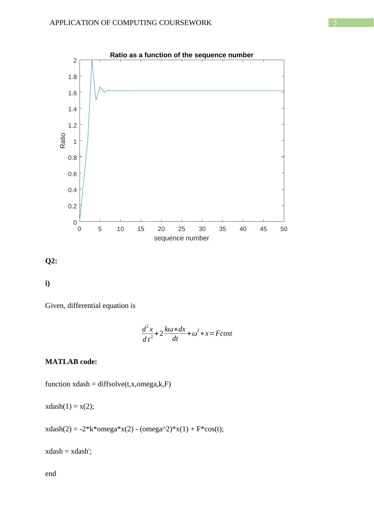
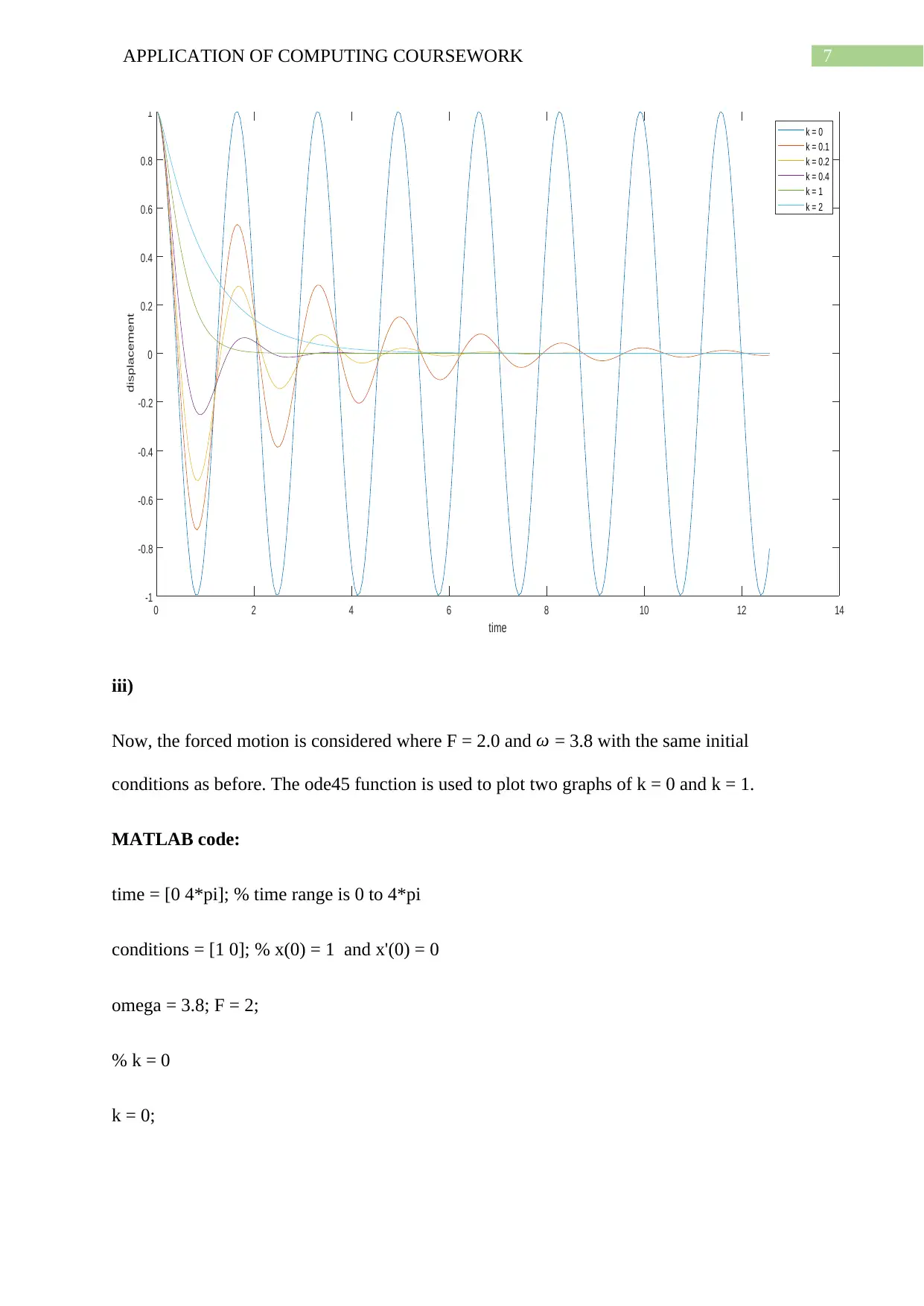
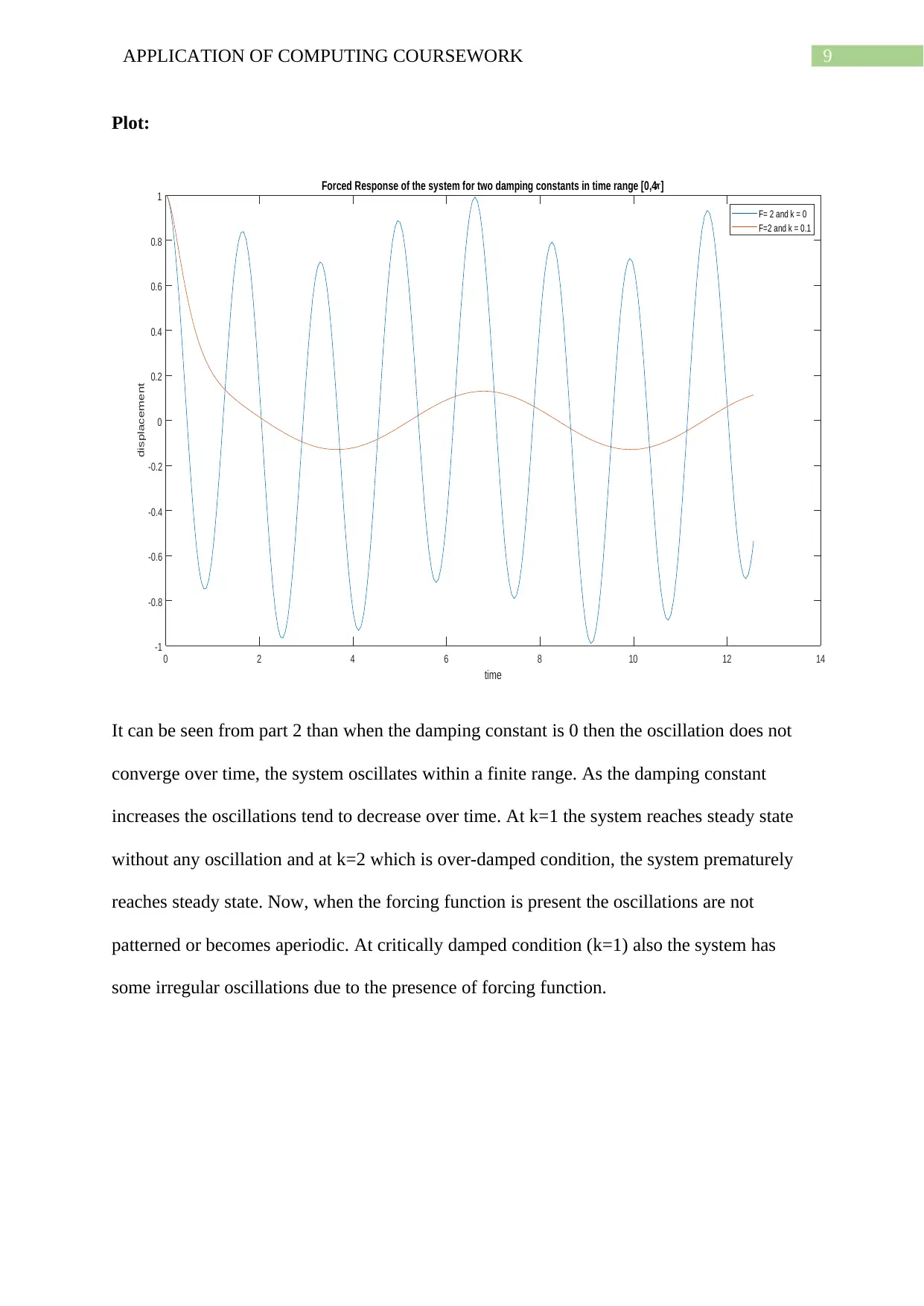
This document presents a complete solution to a computing coursework assignment. The assignment involves two main problems. The first problem requires the computation and analysis of Fibonacci numbers using MATLAB. It includes generating Fibonacci numbers, calculating the ratio of consecutive numbers, plotting the ratio, and determining the smallest value of n for a specified accuracy of the golden mean. The second problem focuses on a mass-spring system subject to damping and a periodic force. It involves solving a differential equation using MATLAB's ode45 function, plotting the system's response for different damping constants, and analyzing the effects of damping on the system's behavior under both unforced and forced conditions. The solution includes MATLAB code, plots, and detailed explanations of the results, demonstrating the application of computing principles to solve engineering problems.

Running head: APPLICATION OF COMPUTING COURSEWORK
APPLICATION OF COMPUTING COURSEWORK
Name of the Student
Name of the University
Author Note

1APPLICATION OF COMPUTING COURSEWORK
Q1:
i) The ratio of Fn/Fn-1 for the first 50 Fibonacci numbers are calculated by the following
MATLAB code.
MATLAB code:
%% Q1 i)
% generating Fibonacci numbers
F(1) = 1; F(2) = 1;
for i=3:50
F(i) = F(i-1) + F(i-2);
end
% computing ratio Fn/Fn-1
n = zeros(1,49);
ratio = zeros(1,49);
for i=2:50
n(i) = i;
ratio(i) = F(i)/F(i-1);
end
%% Q1 ii)
% plotting ratio as a function of n

2APPLICATION OF COMPUTING COURSEWORK
plot(n,ratio)
xlabel('sequence number')
ylabel('Ratio')
title('Ratio as a function of the sequence number')
%% Q1 iii)
i=1;ratio(1)=F(2)/F(1);
g_mean = (1+sqrt(5))/2; % defining golden mean
while (abs(ratio(i)-g_mean)/g_mean)*100 > 0.1 % finding n for which ratio is within 0.1% of
golden mean
i=i+1;
end
sprintf('The smallest value of n=%i for which the ratio is 0.1 percent accurate of golden
mean. The percentage of tolerance is %f',i,(abs(ratio(i)-g_mean)/g_mean)*100)
Output:
fibonacci
ans =
'The smallest value of n=9 for which the ratio is 0.1 percent accurate of golden mean. The
percentage of tolerance is 0.062646'

3APPLICATION OF COMPUTING COURSEWORK
0 5 10 15 20 25 30 35 40 45 50
sequence number
0
0.2
0.4
0.6
0.8
1
1.2
1.4
1.6
1.8
2
Ratio
Ratio as a function of the sequence number
Q2:
i)
Given, differential equation is
d2 x
d t2 + 2 kω∗dx
dt + ω2∗x=Fcost
MATLAB code:
function xdash = diffsolve(t,x,omega,k,F)
xdash(1) = x(2);
xdash(2) = -2*k*omega*x(2) - (omega^2)*x(1) + F*cos(t);
xdash = xdash';
end

4APPLICATION OF COMPUTING COURSEWORK
ii)
The six graphs are plotted with unforced motion F = 0 and ω = 3.8 with initial conditions x(0)
= 1 and x’(0) = 0 by the following MATLAB function.
MATLAB code:
time = [0 4*pi]; % time range is 0 to 4*pi
conditions = [1 0]; % x(0) = 1 and x'(0) = 0
omega = 3.8; F = 0;
% k = 0
k = 0;
[t,x] = ode45(@(t,x) diffsolve(t,x,omega,k,F),time,conditions); % calling ode function
diffsolve
figure(1)
plot(t,x(:,1))
hold on
% k = 0.1
k = 0.1;
[t,x] = ode45(@(t,x) diffsolve(t,x,omega,k,F),time,conditions); % calling ode function
diffsolve
figure(1)
plot(t,x(:,1))

5APPLICATION OF COMPUTING COURSEWORK
hold on
% k = 0.2
k = 0.2;
[t,x] = ode45(@(t,x) diffsolve(t,x,omega,k,F),time,conditions); % calling ode function
diffsolve
figure(1)
plot(t,x(:,1))
hold on
% k = 0.4;
k = 0.4;
[t,x] = ode45(@(t,x) diffsolve(t,x,omega,k,F),time,conditions); % calling ode function
diffsolve
figure(1)
plot(t,x(:,1))
hold on
% k = 1.0
k = 1.0;
[t,x] = ode45(@(t,x) diffsolve(t,x,omega,k,F),time,conditions); % calling ode function
diffsolve

6APPLICATION OF COMPUTING COURSEWORK
figure(1)
plot(t,x(:,1))
hold on
% k = 2.0
k = 2.0;
[t,x] = ode45(@(t,x) diffsolve(t,x,omega,k,F),time,conditions); % calling ode function
diffsolve
figure(1)
plot(t,x(:,1))
xlabel('time')
ylabel('displacement')
legend('k = 0','k = 0.1','k = 0.2','k = 0.4','k = 1','k = 2')
title('Response of the system for different damping constants in time range [0,4\pi]')
Plot:

7APPLICATION OF COMPUTING COURSEWORK
0 2 4 6 8 10 12 14
time
-1
-0.8
-0.6
-0.4
-0.2
0
0.2
0.4
0.6
0.8
1
displacement
Response of the system for different damping constants in time range [0,4 ]
k = 0
k = 0.1
k = 0.2
k = 0.4
k = 1
k = 2
iii)
Now, the forced motion is considered where F = 2.0 and ω = 3.8 with the same initial
conditions as before. The ode45 function is used to plot two graphs of k = 0 and k = 1.
MATLAB code:
time = [0 4*pi]; % time range is 0 to 4*pi
conditions = [1 0]; % x(0) = 1 and x'(0) = 0
omega = 3.8; F = 2;
% k = 0
k = 0;

8APPLICATION OF COMPUTING COURSEWORK
[t,x] = ode45(@(t,x) diffsolve(t,x,omega,k,F),time,conditions); % calling ode function
diffsolve
figure(1)
plot(t,x(:,1))
hold on
% k = 1
k = 1;
[t,x] = ode45(@(t,x) diffsolve(t,x,omega,k,F),time,conditions); % calling ode function
diffsolve
figure(1)
plot(t,x(:,1))
legend('F= 2 and k = 0','F=2 and k = 0.1')
xlabel('time')
ylabel('displacement')
title('Forced Response of the system for two damping constants in time range [0,4\pi]')

9APPLICATION OF COMPUTING COURSEWORK
Plot:
0 2 4 6 8 10 12 14
time
-1
-0.8
-0.6
-0.4
-0.2
0
0.2
0.4
0.6
0.8
1
displacement
Forced Response of the system for two damping constants in time range [0,4 ]
F= 2 and k = 0
F=2 and k = 0.1
It can be seen from part 2 than when the damping constant is 0 then the oscillation does not
converge over time, the system oscillates within a finite range. As the damping constant
increases the oscillations tend to decrease over time. At k=1 the system reaches steady state
without any oscillation and at k=2 which is over-damped condition, the system prematurely
reaches steady state. Now, when the forcing function is present the oscillations are not
patterned or becomes aperiodic. At critically damped condition (k=1) also the system has
some irregular oscillations due to the presence of forcing function.