MATLAB Implementation: Filter Design, Signal Analysis, and BPSK

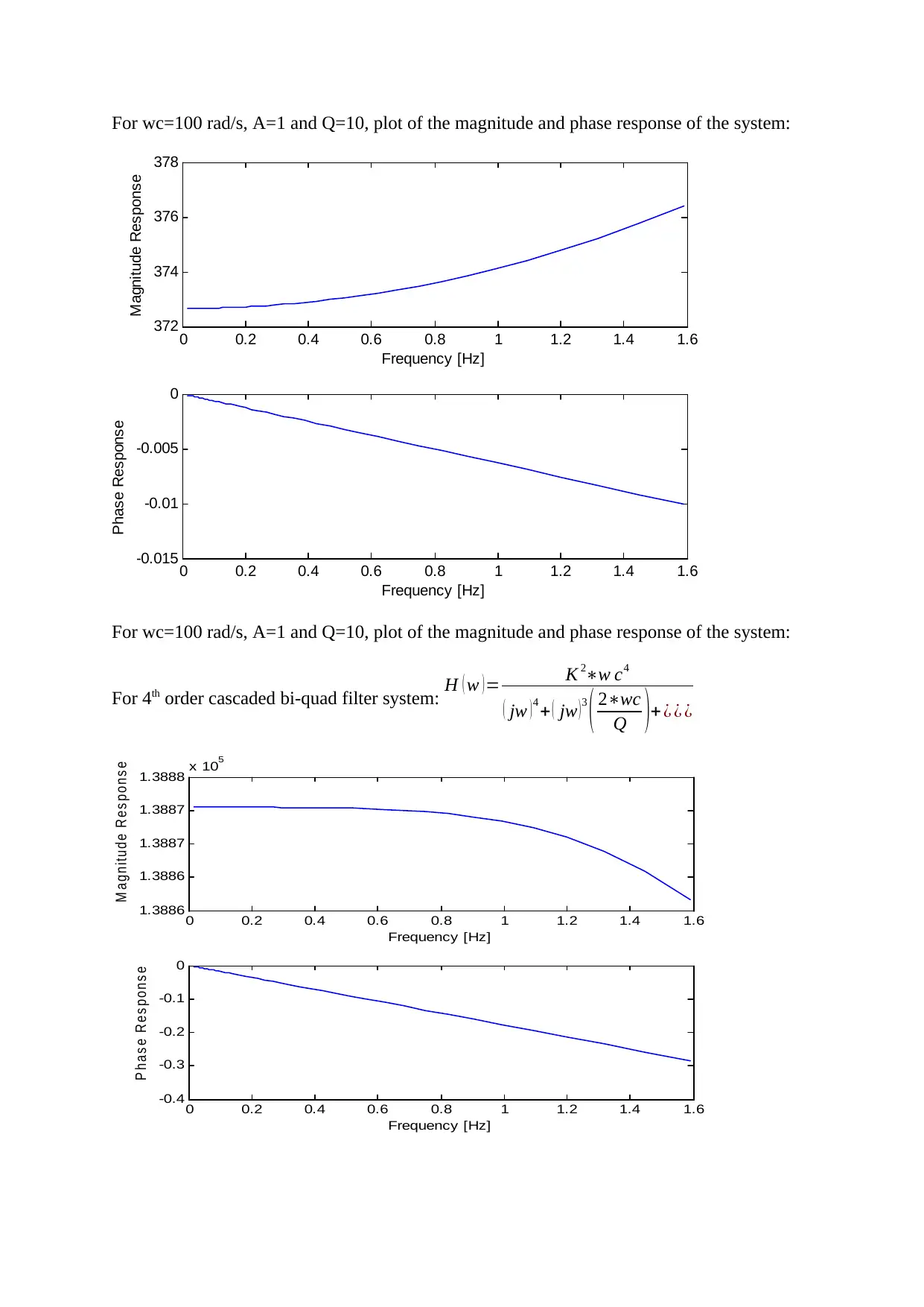
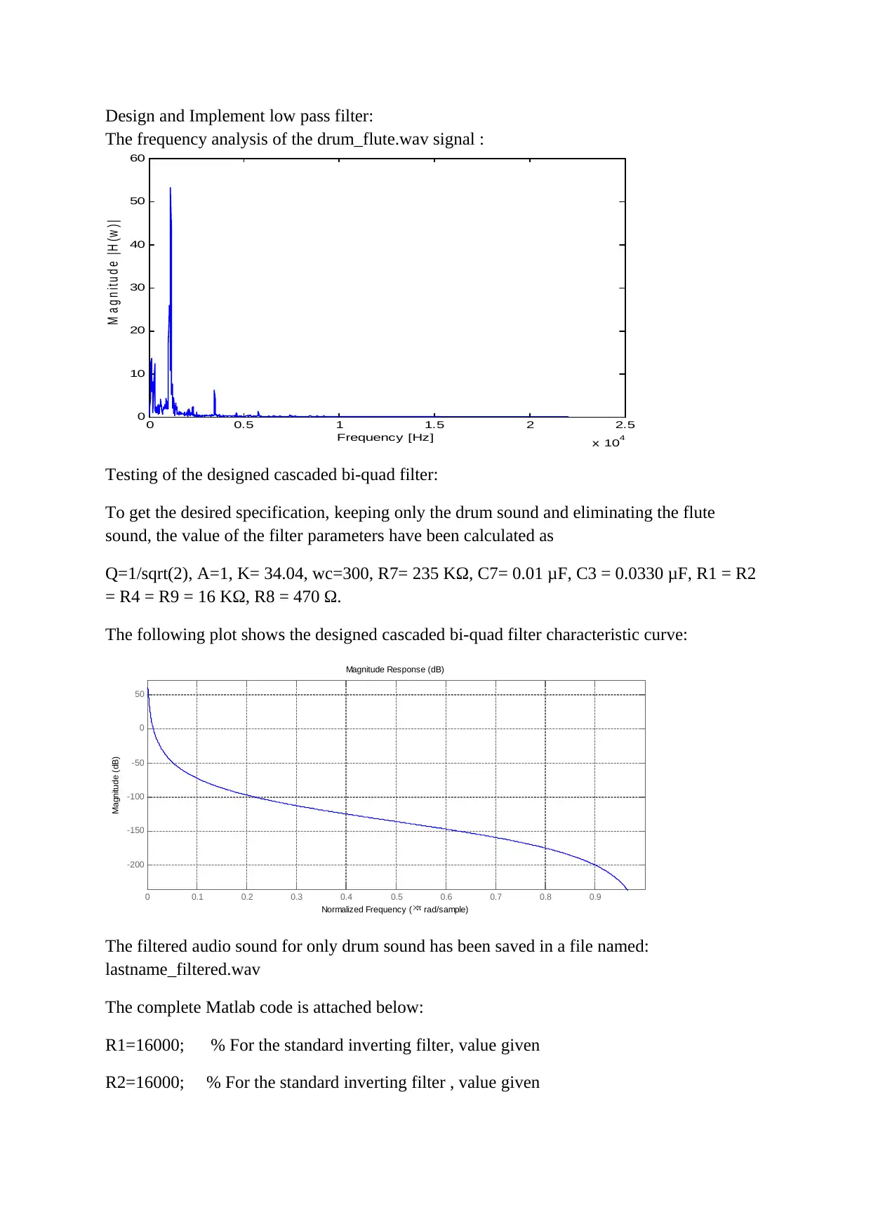
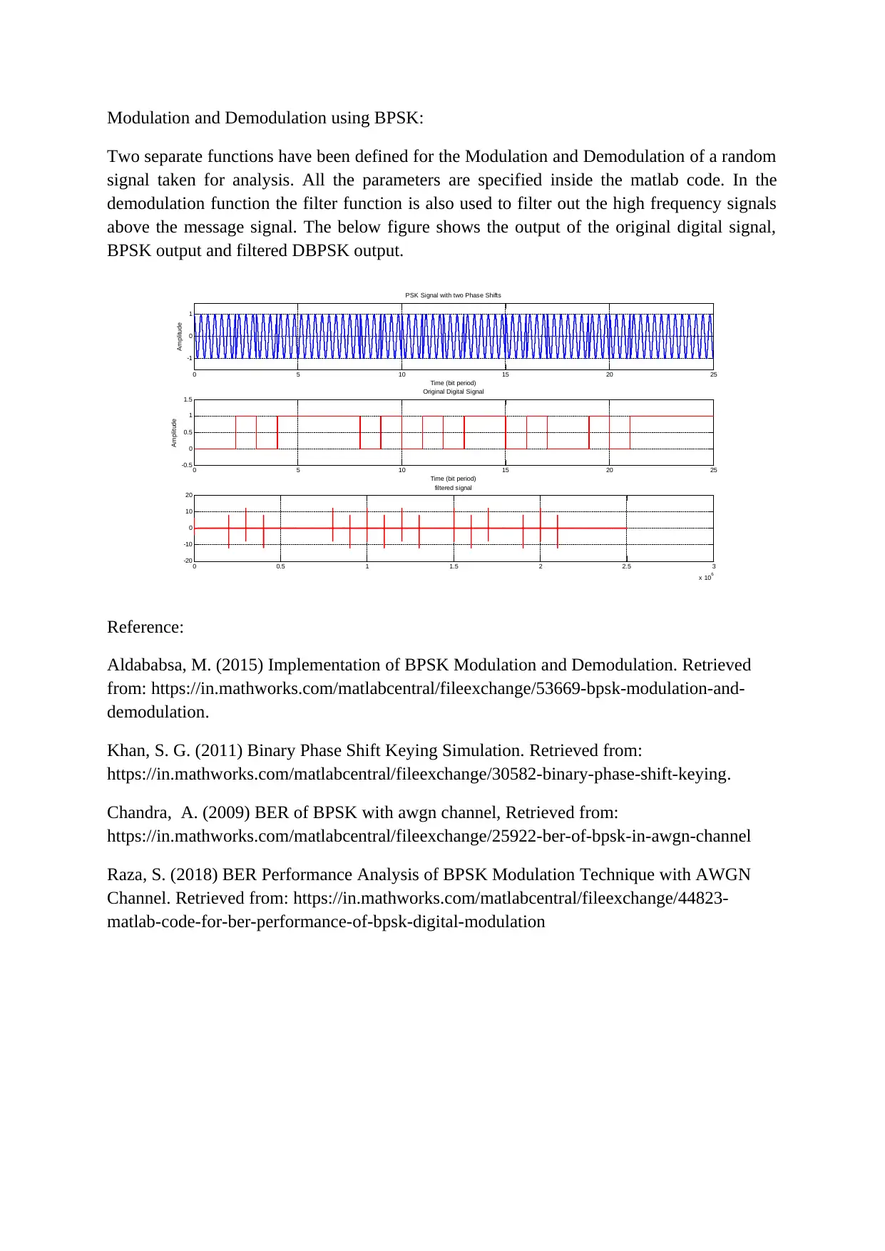
This assignment presents a detailed MATLAB-based solution for several exercises in filter design, signal analysis, and digital communication techniques. The solution includes the design and analysis of various filters, such as inverting filters, integrator filters, and cascaded bi-quad filters, with plots of their magnitude and phase responses. The assignment also covers the frequency analysis of an audio signal and the design of a low-pass filter to isolate specific sounds. Furthermore, it includes the implementation of Binary Phase Shift Keying (BPSK) modulation and demodulation, with plots illustrating the modulated signal and the filtered output. The MATLAB code is provided, including functions for modulation, demodulation, and filter design, along with explanations and references. The student designed and implemented a low pass filter and tested it for the drum_flute.wav signal, providing the filter's characteristic curve and the filtered audio output. The provided solution covers a range of topics in electrical engineering, specifically signal processing and digital communication, offering a practical approach to understanding these concepts.

MATLAB Exercise 1.1: Let R1 = 16 kΩ and R2 = 16 kΩ.
Plot of Magnitude and phase response of the system H ( w )=−R 1
R 2 in frequency domain:
0 0.2 0.4 0.6 0.8 1 1.2 1.4 1.6
0
0.5
1
1.5
2
Frequency [Hz]
Magnitude Response
0 0.2 0.4 0.6 0.8 1 1.2 1.4 1.6
2
3
4
5
Frequency [Hz]
Phase Response
MATLAB Exercise 1.2: Let C3 = 0.033 μF and R4 = 16 kΩ
Plot of Magnitude and phase response of the system H ( w )= −1
jwR 4 C 3 in frequency domain:
0 0.2 0.4 0.6 0.8 1 1.2 1.4 1.6
0
0.5
1
1.5
2 x 104
Frequency [Hz]
Magnitude Response
0 0.2 0.4 0.6 0.8 1 1.2 1.4 1.6
0
1
2
3
Frequency [Hz]
Phase Response

MATLAB Exercise 1.3: Let R7 = 68 kΩ, C7 = 0.01 μF, and R8 = 470Ω.
Plot of Magnitude and phase response of the system H(w)= - R7/R8(1+ jwR7C7) in
frequency domain:
0 0.2 0.4 0.6 0.8 1 1.2 1.4 1.6
0
2
4
6 x 10-3
Frequency [Hz]
Magnitude Response
0 0.2 0.4 0.6 0.8 1 1.2 1.4 1.6
-1.5708
-1.5708
-1.5708
-1.5708
Frequency [Hz]
Phase Response
MATLAB Exercise 1.4:
Let wc = 100 rad/s (≈ 16 Hz), Q = 1/(sqrt2), and A = 1.
Plot of Magnitude and phase response of the system
H(w)= Kwc^2/(-w^2)+jw (wc/Q)+Awc^2 in frequency domain:
0 0.2 0.4 0.6 0.8 1 1.2 1.4 1.6
372.64
372.645
372.65
372.655
372.66
Frequency [Hz]
M a g n i t u d e R e s p o n s e
0 0.2 0.4 0.6 0.8 1 1.2 1.4 1.6
-0.2
-0.15
-0.1
-0.05
0
Frequency [Hz]
P h a s e R e s p o n s e

For wc = 50 rad/s and the value of Q, A keeping constant, plot of the magnitude and phase
response of the system
0 0.2 0.4 0.6 0.8 1 1.2 1.4 1.6
372.3
372.4
372.5
372.6
372.7
Frequency [Hz]
Magnitude Response
0 0.2 0.4 0.6 0.8 1 1.2 1.4 1.6
-0.4
-0.3
-0.2
-0.1
0
Frequency [Hz]
Phase Response
For wc = 200 rad/s and the value of Q, A keeping constant, plot of the magnitude and phase
response of the system
0 0.2 0.4 0.6 0.8 1 1.2 1.4 1.6
372.6585
372.659
372.6595
372.66
372.6605
Frequency [Hz]
M a g n it u d e R e s p o n s e
0 0.2 0.4 0.6 0.8 1 1.2 1.4 1.6
-0.08
-0.06
-0.04
-0.02
0
Frequency [Hz]
P h a s e R e s p o n s e

For wc=100 rad/s, A=1 and Q=0.1 plot of the magnitude and phase response of the system
0 0.2 0.4 0.6 0.8 1 1.2 1.4 1.6
250
300
350
400
Frequency [Hz]
Magnitude Response
0 0.2 0.4 0.6 0.8 1 1.2 1.4 1.6
-0.8
-0.6
-0.4
-0.2
0
Frequency [Hz]
Phase Response
For wc=100 rad/s, A keeping constant and Q=1 plot of the magnitude and phase response of
the system:
0 0.2 0.4 0.6 0.8 1 1.2 1.4 1.6
372
373
374
375
Frequency [Hz]
Magnitude Response
0 0.2 0.4 0.6 0.8 1 1.2 1.4 1.6
-0.2
-0.15
-0.1
-0.05
0
Frequency [Hz]
Phase Response

For wc=100 rad/s, A=1 and Q=10, plot of the magnitude and phase response of the system:
0 0.2 0.4 0.6 0.8 1 1.2 1.4 1.6
372
374
376
378
Frequency [Hz]
Magnitude Response
0 0.2 0.4 0.6 0.8 1 1.2 1.4 1.6
-0.015
-0.01
-0.005
0
Frequency [Hz]
Phase Response
For wc=100 rad/s, A=1 and Q=10, plot of the magnitude and phase response of the system:
For 4th order cascaded bi-quad filter system: H ( w ) = K 2∗w c4
( jw ) 4 + ( jw ) 3
( 2∗wc
Q )+ ¿ ¿ ¿
0 0.2 0.4 0.6 0.8 1 1.2 1.4 1.6
1.3886
1.3886
1.3887
1.3887
1.3888 x 10
5
Frequency [Hz]
M a gn itu de R es po ns e
0 0.2 0.4 0.6 0.8 1 1.2 1.4 1.6
-0.4
-0.3
-0.2
-0.1
0
Frequency [Hz]
P h as e R e s p on s e

Design and Implement low pass filter:
The frequency analysis of the drum_flute.wav signal :
0 0.5 1 1.5 2 2.5
x 10
4
0
10
20
30
40
50
60
Frequency [Hz]
M a g n i t u d e |H (w ) |
Testing of the designed cascaded bi-quad filter:
To get the desired specification, keeping only the drum sound and eliminating the flute
sound, the value of the filter parameters have been calculated as
Q=1/sqrt(2), A=1, K= 34.04, wc=300, R7= 235 KΩ, C7= 0.01 μF, C3 = 0.0330 μF, R1 = R2
= R4 = R9 = 16 KΩ, R8 = 470 Ω.
The following plot shows the designed cascaded bi-quad filter characteristic curve:
0 0.1 0.2 0.3 0.4 0.5 0.6 0.7 0.8 0.9
-200
-150
-100
-50
0
50
Normalized Frequency ( rad/sample)
Magnitude (dB)
Magnitude Response (dB)
The filtered audio sound for only drum sound has been saved in a file named:
lastname_filtered.wav
The complete Matlab code is attached below:
R1=16000; % For the standard inverting filter, value given
R2=16000; % For the standard inverting filter , value given

%num=[-R1]; % numerator of inverting filter frequency response
%den=[R2]; % denomenator of inverting filter frequency response
R4= 16000; %For the integrator inverting filter, value given
c3=0.0330*10^-6; %For the integrator inverting filter, value given
%num=[0 -1]; % numerator of integrator inverting filter frequency response
%den=[R4*c3 0]; % denomenator of integrator inverting filter frequency response
%R7= 68000; %For the integrator inverting filter with decay, value given
R8= 470; %For the integrator inverting filter with decay, value given
c7= 0.01*10^-6; %For the integrator inverting filter with decay, value given
R7=235000; %For the cascaded bi-quad filter, value calculated
%num=[0 -(R7/R8)]; % numerator of integrator inverting filter with decay frequency
response
%den=[(R7*c7) 1 ]; % denomenator of integrator inverting filter with decay frequency
response
k=372.66; %costant for biquad cascaded filter, value calculated
wc=100; wc=50; wc=200;
k=34.04; %costant for biquad cascaded filter used for only drum sound, value calculated
wc=300; % wc value for biquad cascaded filter used for only drum sound, value
calculated
A=1;
Q=1/sqrt(2);
%Q=10;
%num=[0 0 (k*wc^2)]; % numerator of single bi-quad filter frequency response
%den=[1 (wc/Q) (A*wc^2)]; % denomenator of single bi-quad filter frequency response
num=[0 0 0 0 ((k*wc^2)^2)]; % numerator of cascaded bi-quad filter frequency
response
den=[1 2*(wc/Q) ((2*A*wc^2)+(wc/Q)^2) ((2*A*(wc)^3)/Q) ((A^2)*(wc)^4)]; %
denomenator of cascaded bi-quad filter frequency response

h=tf(num,den) %transfer function of cascaded bi-quad filter frequency
response
[y,Fs] = audioread('drum_flute.wav') % to read the audio file % y = data vector of audio %
Fs= sampling frequency
%ffty=fft(y); % fft of y for freq analysis
%Nfft=2048; % length of y
%f=linspace(0,Fs,Nfft); %to initialize the x axis, frequency domain
%G=abs(fft(y,Nfft)); %Absolute value of fft y
%figure;
%plot(f(1:Nfft/2),G(1:Nfft/2)) % plot of fft
%xlabel('Frequency [Hz]'); ylabel('Magnitude |H(w)|')
%w=logspace(-1,1); % to initialize the x axis
%H = freqs(num,den,w); %fequency analysis of cascaded filter
%y= abs(H); % absolute value of H
%x=angle(H); %angle of H
%subplot(211);
%plot(w,abs(H));
%plot(w/(2*pi), abs(H)); % plot of frequency in hz and magnitude of H
%xlabel('Frequency [Hz]'); ylabel('Magnitude Response');
%subplot(212);
%plot(w/(2*pi),x);
%xlabel('Frequency [Hz]'); ylabel('Phase Response');
[numd,dend] = bilinear(num,den,Fs) % to convert the analog filter to digital
fvtool(numd,dend) %to to get the filter characteristic curve

y_filtered = filter(numd,dend,y)% Implement Digital filter and y_filtered= filtered output of
y, audio signal
sound(y_filtered,Fs) % produce filtered audio
audiowrite('lastname_filtered.wav',y_filtered,Fs) %to save filtered audio in
lastname_filtered.wav
NFFT=2048;
f=linspace(0,Fs,NFFT);
G=abs(fft(y_filtered,NFFT));
figure;
plot(f(1:NFFT/2),G(1:NFFT/2)) %to get the fft of filtered audio

Modulation and Demodulation using BPSK:
Two separate functions have been defined for the Modulation and Demodulation of a random
signal taken for analysis. All the parameters are specified inside the matlab code. In the
demodulation function the filter function is also used to filter out the high frequency signals
above the message signal. The below figure shows the output of the original digital signal,
BPSK output and filtered DBPSK output.
0 5 10 15 20 25
-1
0
1
Time (bit period)
Amplitude
PSK Signal with two Phase Shifts
0 5 10 15 20 25
-0.5
0
0.5
1
1.5
Time (bit period)
Amplitude
Original Digital Signal
0 0.5 1 1.5 2 2.5 3
x 106
-20
-10
0
10
20
filtered signal
Reference:
Aldababsa, M. (2015) Implementation of BPSK Modulation and Demodulation. Retrieved
from: https://in.mathworks.com/matlabcentral/fileexchange/53669-bpsk-modulation-and-
demodulation.
Khan, S. G. (2011) Binary Phase Shift Keying Simulation. Retrieved from:
https://in.mathworks.com/matlabcentral/fileexchange/30582-binary-phase-shift-keying.
Chandra, A. (2009) BER of BPSK with awgn channel, Retrieved from:
https://in.mathworks.com/matlabcentral/fileexchange/25922-ber-of-bpsk-in-awgn-channel
Raza, S. (2018) BER Performance Analysis of BPSK Modulation Technique with AWGN
Channel. Retrieved from: https://in.mathworks.com/matlabcentral/fileexchange/44823-
matlab-code-for-ber-performance-of-bpsk-digital-modulation