MATLAB Coding and Analysis of Residential Load Disaggregation Project

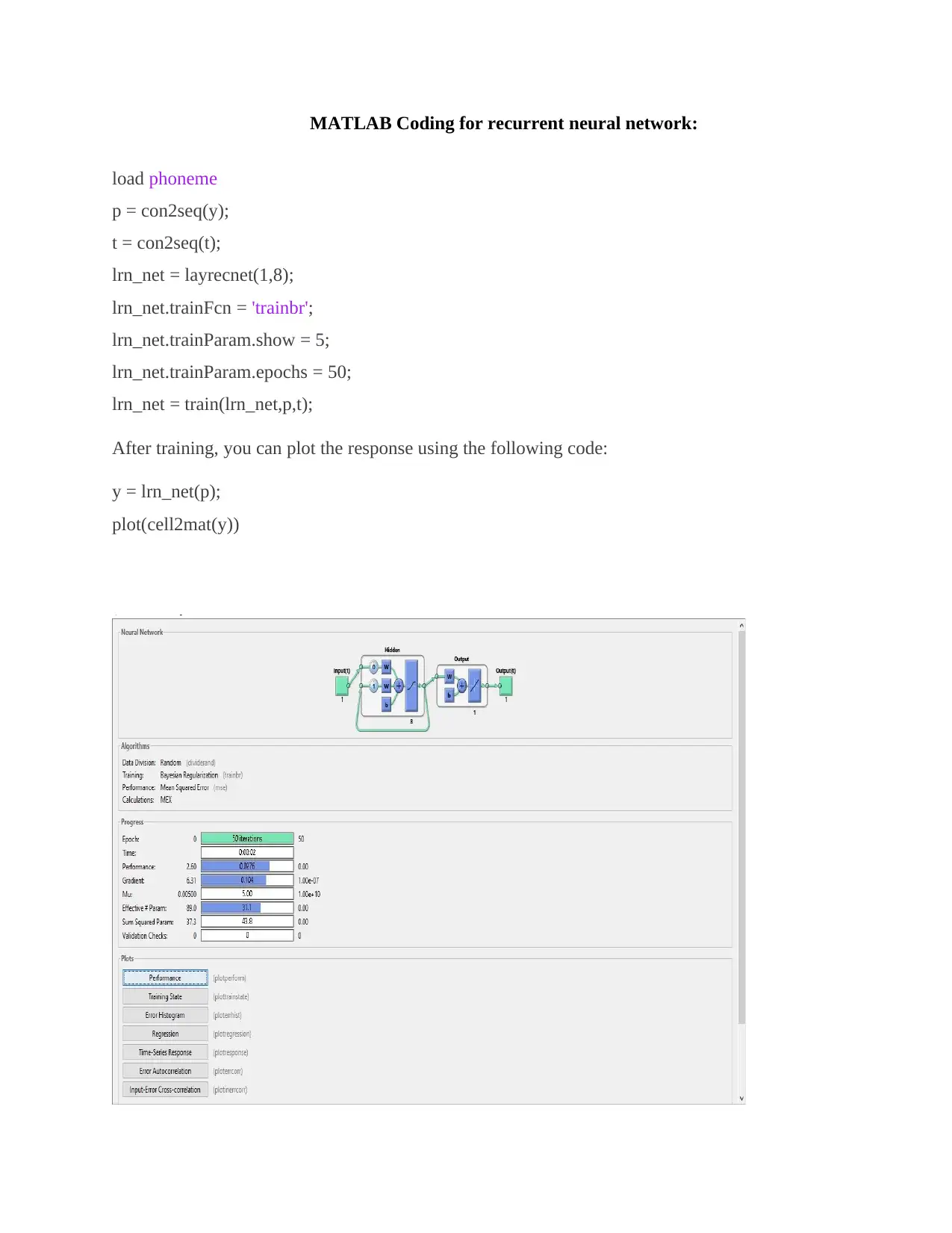
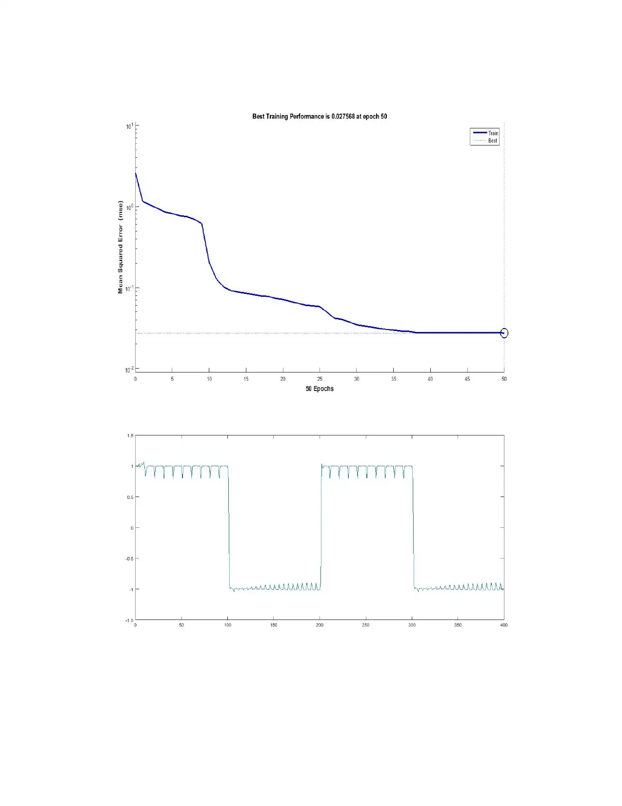
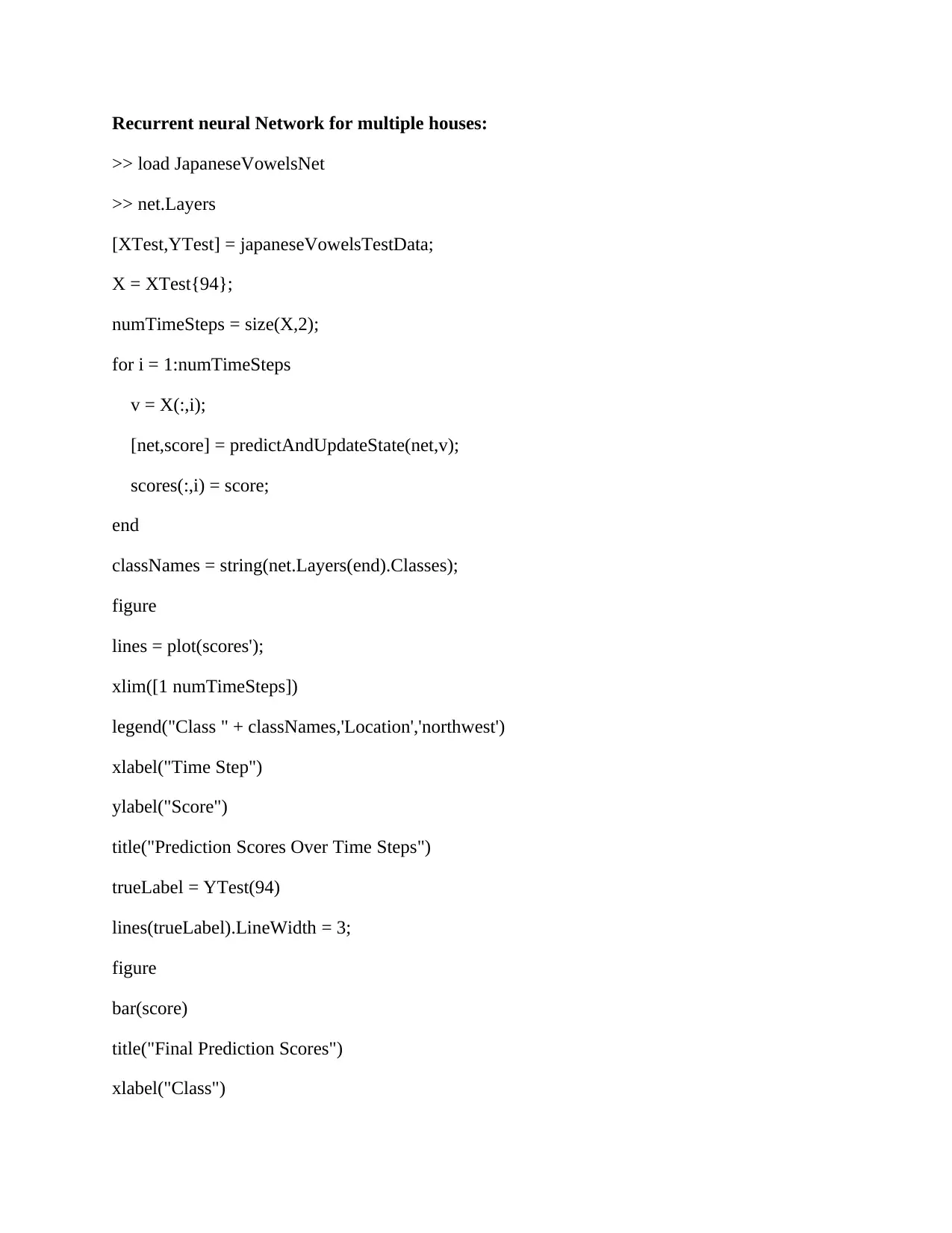
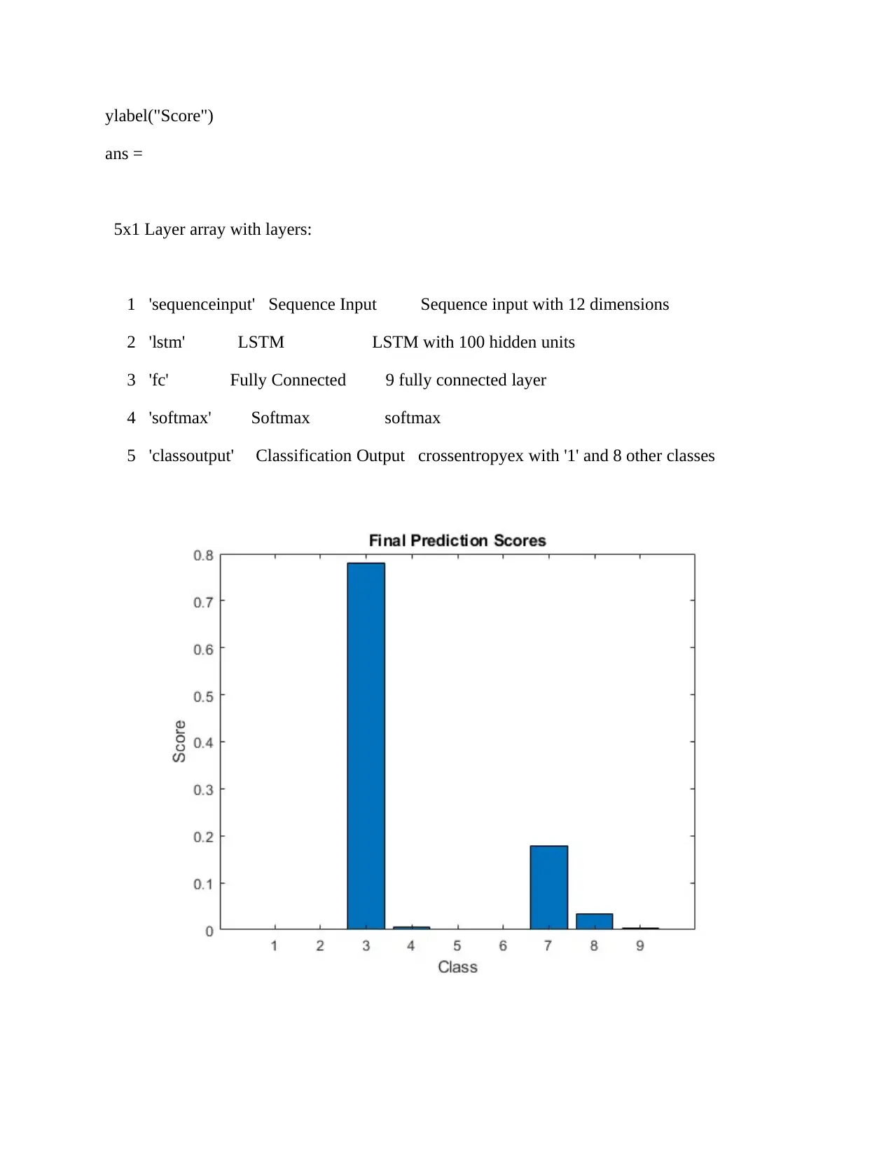
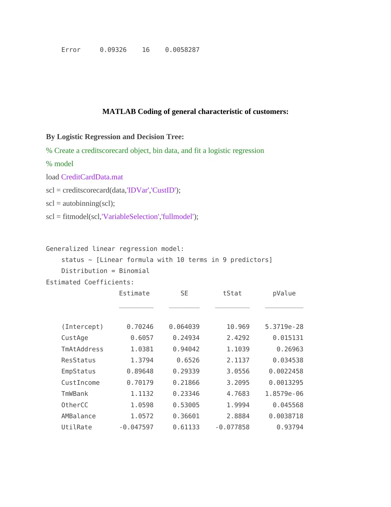
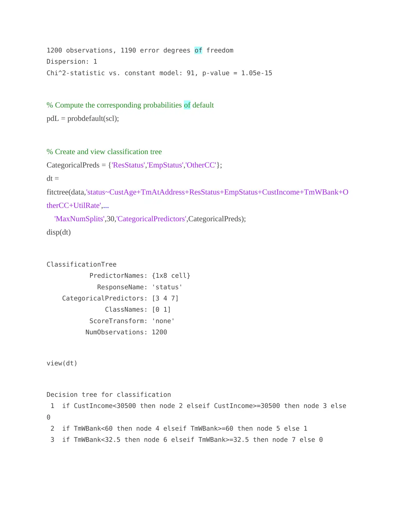
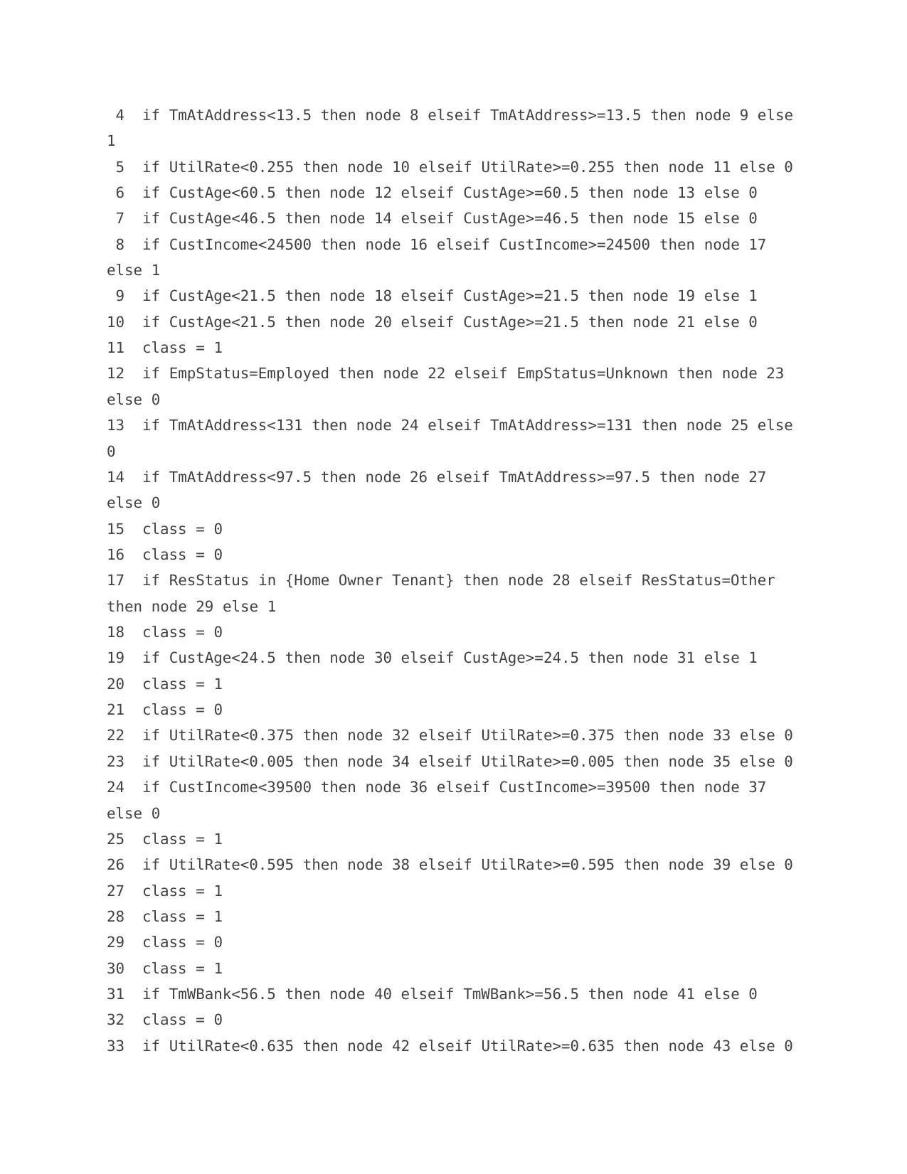
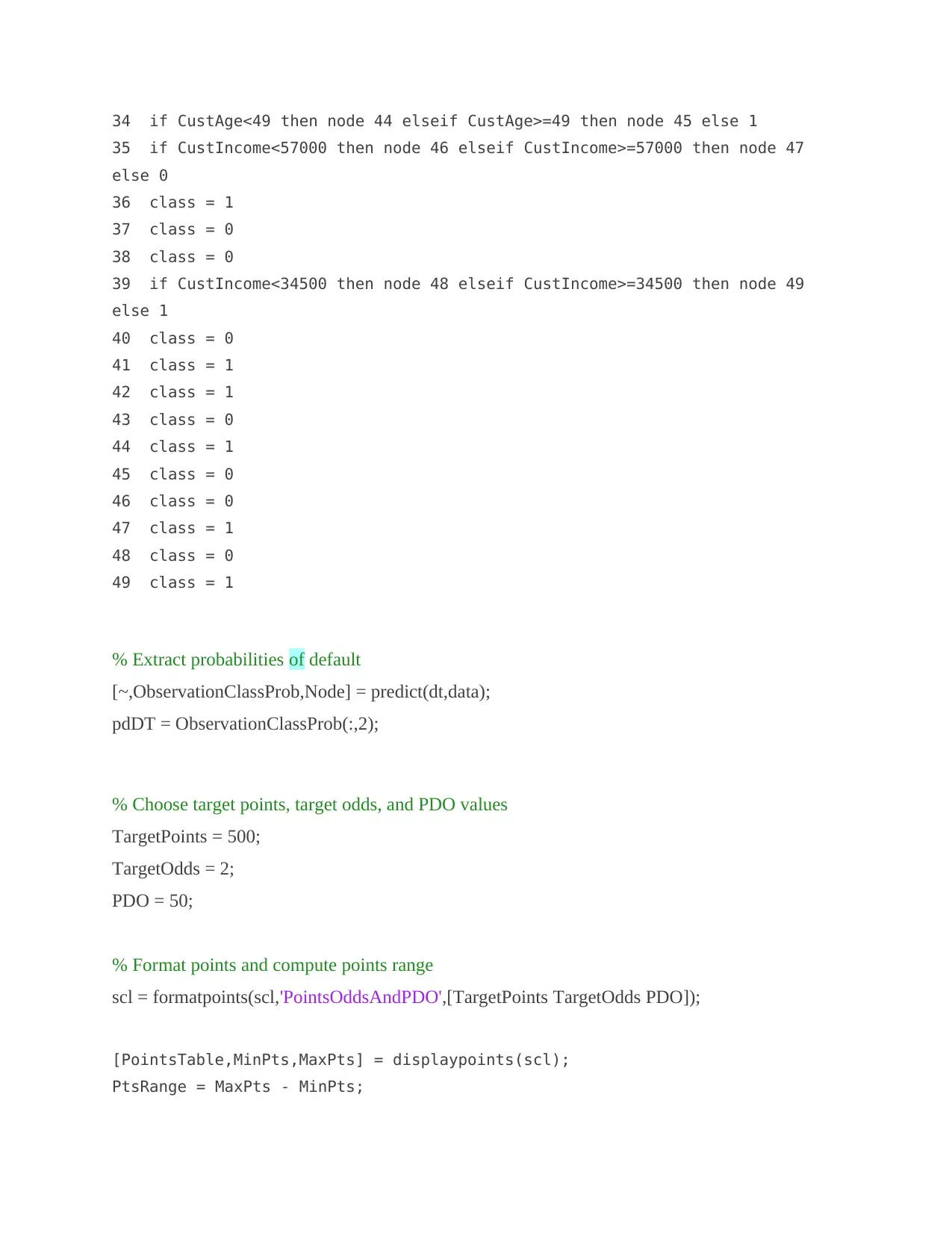
This MATLAB project focuses on disaggregating residential load profiles, a critical aspect of smart grid technology and energy management. The assignment includes MATLAB code examples demonstrating various techniques, including recurrent neural networks for time series regression and customer characteristic analysis using logistic regression and decision trees. The project explores the effects of external factors on aggregated load profiles and utilizes the EDHMM-diff technique to model individual home appliance loads, simulating and verifying the model in MATLAB. The provided code covers diverse applications, such as air conditioner detection and data aggregation analysis, to provide a comprehensive understanding of residential load disaggregation and its practical implementation. The project also presents examples of credit risk assessment and monitoring system prototypes.

MATLAB Coding for recurrent neural network:
load phoneme
p = con2seq(y);
t = con2seq(t);
lrn_net = layrecnet(1,8);
lrn_net.trainFcn = 'trainbr';
lrn_net.trainParam.show = 5;
lrn_net.trainParam.epochs = 50;
lrn_net = train(lrn_net,p,t);
After training, you can plot the response using the following code:
y = lrn_net(p);
plot(cell2mat(y))

Recurrent neural Network for multiple houses:
>> load JapaneseVowelsNet
>> net.Layers
[XTest,YTest] = japaneseVowelsTestData;
X = XTest{94};
numTimeSteps = size(X,2);
for i = 1:numTimeSteps
v = X(:,i);
[net,score] = predictAndUpdateState(net,v);
scores(:,i) = score;
end
classNames = string(net.Layers(end).Classes);
figure
lines = plot(scores');
xlim([1 numTimeSteps])
legend("Class " + classNames,'Location','northwest')
xlabel("Time Step")
ylabel("Score")
title("Prediction Scores Over Time Steps")
trueLabel = YTest(94)
lines(trueLabel).LineWidth = 3;
figure
bar(score)
title("Final Prediction Scores")
xlabel("Class")

ylabel("Score")
ans =
5x1 Layer array with layers:
1 'sequenceinput' Sequence Input Sequence input with 12 dimensions
2 'lstm' LSTM LSTM with 100 hidden units
3 'fc' Fully Connected 9 fully connected layer
4 'softmax' Softmax softmax
5 'classoutput' Classification Output crossentropyex with '1' and 8 other classes

MATLAB Coding for regress Start Time, End Time and power average algorithm:
TIME SERIES REGRESSION:
load Data_CreditDefaults
X0 = Data(:,1:4); % Initial predictor set (matrix)
X0Tbl = DataTable(:,1:4); % Initial predictor set (tabular array)
predNames0 = series(1:4); % Initial predictor set names
T0 = size(X0,1); % Sample size
y0 = Data(:,5); % Response data
respName0 = series{5}; % Response data name
% Convert dates to serial date numbers:
dateNums = datenum([dates,ones(T0,2)]);
% Plot potential predictors:
figure;
plot(dateNums,X0,'LineWidth',2)
ax = gca;
ax.XTick = dateNums(1:2:end);
datetick('x','yyyy','keepticks')
recessionplot;
xlabel('Year')
ylabel('Predictor Level')
legend(predNames0,'Location','NW')
title('{\bf Potential Predictors}')
axis('tight')
grid('on')

% Plot response:
figure;
hold('on');
plot(dateNums,y0,'k','LineWidth',2);
plot(dateNums,y0-detrend(y0),'m--')
hold('off');
ax = gca;
ax.XTick = dateNums(1:2:end);
datetick('x','yyyy','keepticks')
recessionplot;
xlabel('Year')
ylabel('Response Level')
legend(respName0,'Linear Trend','Location','NW')
title('{\bf Response}')
axis('tight');

grid('on');
% Add intercept to model:
X0I = [ones(T0,1),X0]; % Matrix
X0ITbl = [table(ones(T0,1),'VariableNames',{'Const'}),X0Tbl]; % Table
Estimate = X0I\y0
Estimate = 5×1
-0.2274

0.0168
0.0043
-0.0149
0.0455
M0 = fitlm(DataTable)
M0 =
Linear regression model:
IGD ~ 1 + AGE + BBB + CPF + SPR
Estimated Coefficients:
Estimate SE tStat pValue
_________ _________ _______ _________
(Intercept) -0.22741 0.098565 -2.3072 0.034747
AGE 0.016781 0.0091845 1.8271 0.086402
BBB 0.0042728 0.0026757 1.5969 0.12985
CPF -0.014888 0.0038077 -3.91 0.0012473
SPR 0.045488 0.033996 1.338 0.1996
Number of observations: 21, Error degrees of freedom: 16
Root Mean Squared Error: 0.0763
R-squared: 0.621, Adjusted R-Squared: 0.526
F-statistic vs. constant model: 6.56, p-value = 0.00253
ANOVATable = anova(M0)
ANOVATable=5×5 table
SumSq DF MeanSq F pValue
________ __ _________ ______ _________
AGE 0.019457 1 0.019457 3.3382 0.086402
BBB 0.014863 1 0.014863 2.55 0.12985
CPF 0.089108 1 0.089108 15.288 0.0012473
SPR 0.010435 1 0.010435 1.7903 0.1996

Error 0.09326 16 0.0058287
MATLAB Coding of general characteristic of customers:
By Logistic Regression and Decision Tree:
% Create a creditscorecard object, bin data, and fit a logistic regression
% model
load CreditCardData.mat
scl = creditscorecard(data,'IDVar','CustID');
scl = autobinning(scl);
scl = fitmodel(scl,'VariableSelection','fullmodel');
Generalized linear regression model:
status ~ [Linear formula with 10 terms in 9 predictors]
Distribution = Binomial
Estimated Coefficients:
Estimate SE tStat pValue
_________ ________ _________ __________
(Intercept) 0.70246 0.064039 10.969 5.3719e-28
CustAge 0.6057 0.24934 2.4292 0.015131
TmAtAddress 1.0381 0.94042 1.1039 0.26963
ResStatus 1.3794 0.6526 2.1137 0.034538
EmpStatus 0.89648 0.29339 3.0556 0.0022458
CustIncome 0.70179 0.21866 3.2095 0.0013295
TmWBank 1.1132 0.23346 4.7683 1.8579e-06
OtherCC 1.0598 0.53005 1.9994 0.045568
AMBalance 1.0572 0.36601 2.8884 0.0038718
UtilRate -0.047597 0.61133 -0.077858 0.93794

1200 observations, 1190 error degrees of freedom
Dispersion: 1
Chi^2-statistic vs. constant model: 91, p-value = 1.05e-15
% Compute the corresponding probabilities of default
pdL = probdefault(scl);
% Create and view classification tree
CategoricalPreds = {'ResStatus','EmpStatus','OtherCC'};
dt =
fitctree(data,'status~CustAge+TmAtAddress+ResStatus+EmpStatus+CustIncome+TmWBank+O
therCC+UtilRate',...
'MaxNumSplits',30,'CategoricalPredictors',CategoricalPreds);
disp(dt)
ClassificationTree
PredictorNames: {1x8 cell}
ResponseName: 'status'
CategoricalPredictors: [3 4 7]
ClassNames: [0 1]
ScoreTransform: 'none'
NumObservations: 1200
view(dt)
Decision tree for classification
1 if CustIncome<30500 then node 2 elseif CustIncome>=30500 then node 3 else
0
2 if TmWBank<60 then node 4 elseif TmWBank>=60 then node 5 else 1
3 if TmWBank<32.5 then node 6 elseif TmWBank>=32.5 then node 7 else 0

4 if TmAtAddress<13.5 then node 8 elseif TmAtAddress>=13.5 then node 9 else
1
5 if UtilRate<0.255 then node 10 elseif UtilRate>=0.255 then node 11 else 0
6 if CustAge<60.5 then node 12 elseif CustAge>=60.5 then node 13 else 0
7 if CustAge<46.5 then node 14 elseif CustAge>=46.5 then node 15 else 0
8 if CustIncome<24500 then node 16 elseif CustIncome>=24500 then node 17
else 1
9 if CustAge<21.5 then node 18 elseif CustAge>=21.5 then node 19 else 1
10 if CustAge<21.5 then node 20 elseif CustAge>=21.5 then node 21 else 0
11 class = 1
12 if EmpStatus=Employed then node 22 elseif EmpStatus=Unknown then node 23
else 0
13 if TmAtAddress<131 then node 24 elseif TmAtAddress>=131 then node 25 else
0
14 if TmAtAddress<97.5 then node 26 elseif TmAtAddress>=97.5 then node 27
else 0
15 class = 0
16 class = 0
17 if ResStatus in {Home Owner Tenant} then node 28 elseif ResStatus=Other
then node 29 else 1
18 class = 0
19 if CustAge<24.5 then node 30 elseif CustAge>=24.5 then node 31 else 1
20 class = 1
21 class = 0
22 if UtilRate<0.375 then node 32 elseif UtilRate>=0.375 then node 33 else 0
23 if UtilRate<0.005 then node 34 elseif UtilRate>=0.005 then node 35 else 0
24 if CustIncome<39500 then node 36 elseif CustIncome>=39500 then node 37
else 0
25 class = 1
26 if UtilRate<0.595 then node 38 elseif UtilRate>=0.595 then node 39 else 0
27 class = 1
28 class = 1
29 class = 0
30 class = 1
31 if TmWBank<56.5 then node 40 elseif TmWBank>=56.5 then node 41 else 0
32 class = 0
33 if UtilRate<0.635 then node 42 elseif UtilRate>=0.635 then node 43 else 0

34 if CustAge<49 then node 44 elseif CustAge>=49 then node 45 else 1
35 if CustIncome<57000 then node 46 elseif CustIncome>=57000 then node 47
else 0
36 class = 1
37 class = 0
38 class = 0
39 if CustIncome<34500 then node 48 elseif CustIncome>=34500 then node 49
else 1
40 class = 0
41 class = 1
42 class = 1
43 class = 0
44 class = 1
45 class = 0
46 class = 0
47 class = 1
48 class = 0
49 class = 1
% Extract probabilities of default
[~,ObservationClassProb,Node] = predict(dt,data);
pdDT = ObservationClassProb(:,2);
% Choose target points, target odds, and PDO values
TargetPoints = 500;
TargetOdds = 2;
PDO = 50;
% Format points and compute points range
scl = formatpoints(scl,'PointsOddsAndPDO',[TargetPoints TargetOdds PDO]);
[PointsTable,MinPts,MaxPts] = displaypoints(scl);
PtsRange = MaxPts - MinPts;