2018 Computer Application for Mechanical Engineering MATLAB Solutions

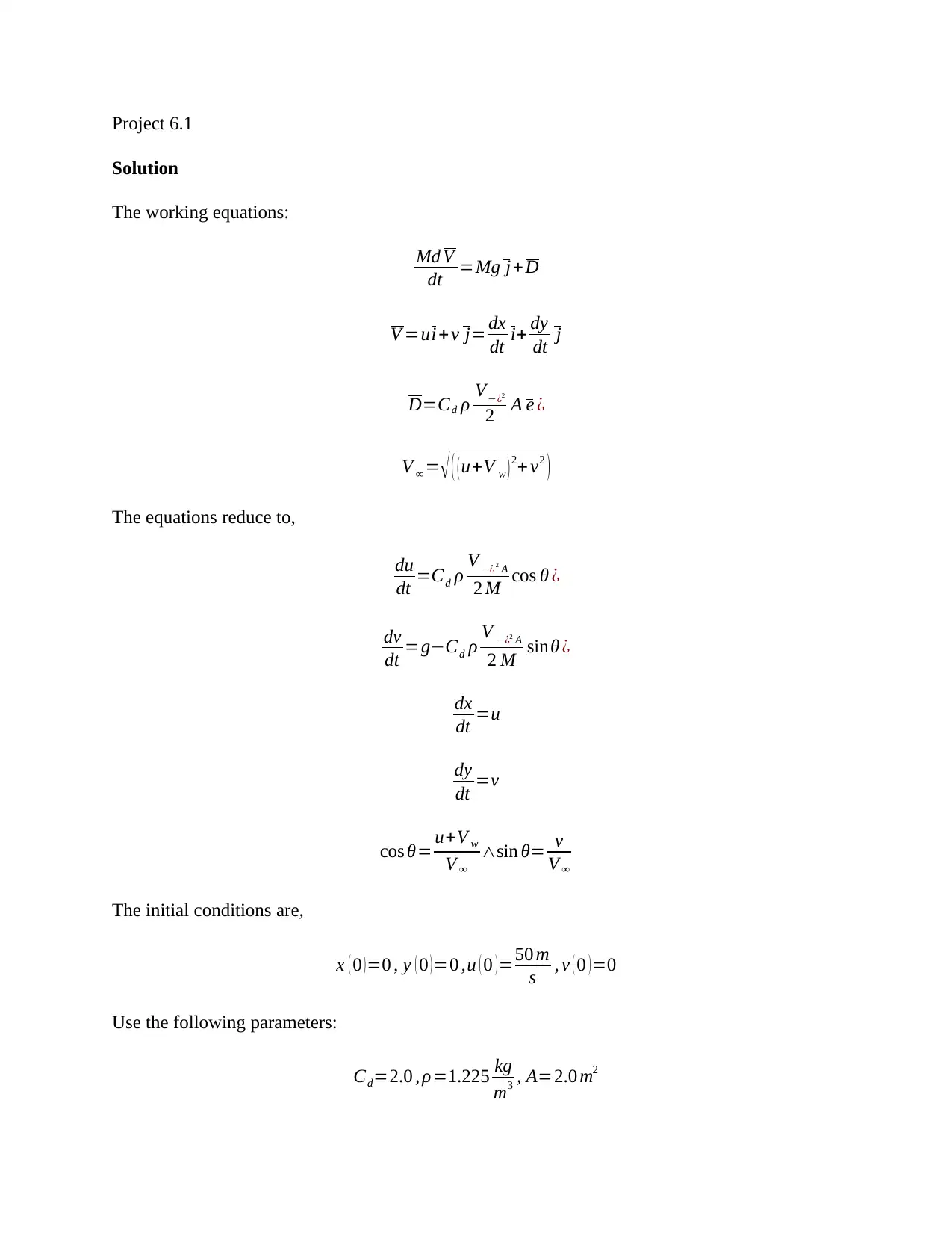
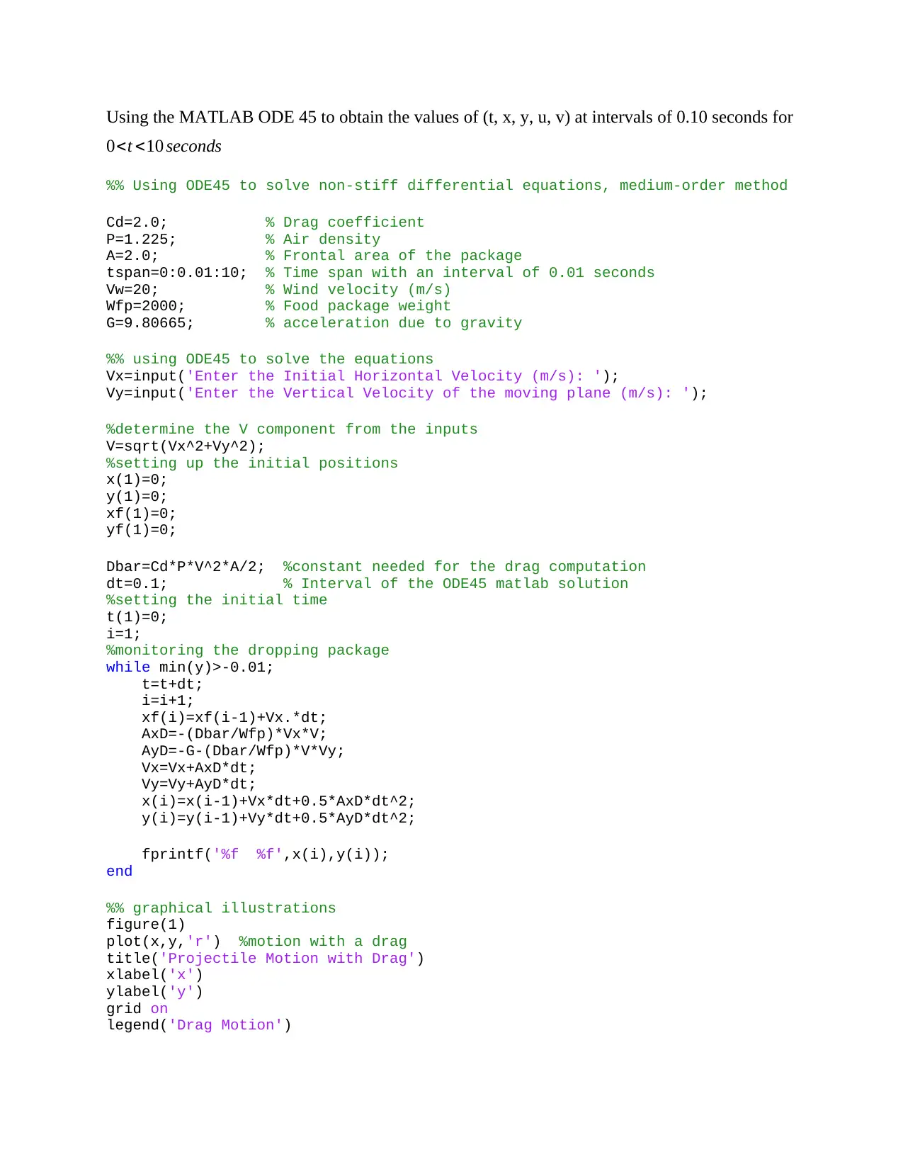
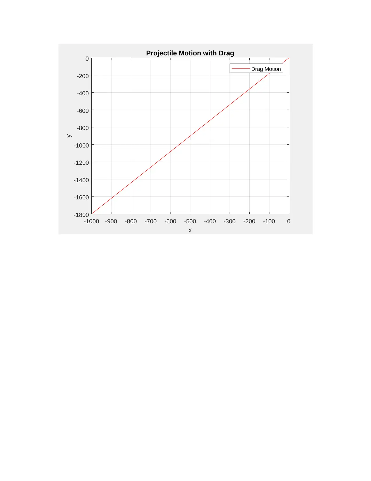
This document presents MATLAB solutions for two mechanical engineering problems. The first problem involves filling a table using MATLAB, related to heat transfer, and discusses using search methods to find real roots of a function, along with convection boundary conditions in Cartesian coordinates. It includes a MATLAB script for temperature simulation. The second problem uses MATLAB's ODE45 solver to determine the trajectory of a projectile with drag, providing equations of motion and initial conditions, and includes a MATLAB script to solve the differential equations and generate a plot of the projectile's motion. Desklib offers many such assignments and study tools.

2018
Computer Application for Mechanical Engineering
United States
Institutional Affiliation
Student name
Student ID number
Date of Submission

Project 4.2
Solution
Use MATLAB to fill in the following table,
X(min) \ T(C) 15 20 25 30
0.1 620.6897 416.6667 382.9787 375.0000
0.2 641.6639 430.7466 395.9203 387.6720
0.3 660.1080 443.1281 407.3007 398.8153
0.4 673.7973 452.3176 415.7473 407.0859
0.5 681.0810 457.2072 420.2415 411.4865
0.6 681.0810 457.2072 420.2415 411.4865
0.7 673.7973 452.3176 415.7473 407.0859
0.8 660.1080 443.1281 407.3007 398.8153
0.9 641.6639 430.7466 395.9203 387.6720
1.0 620.6897 416.6667 382.9787 375.0000
Using the search method, the function must be written in the form,
f ( x )=0
Perform a search to obtain the intervals in which the real roots lie. Sub-divide the x domain into
N equal subdivisions, giving,
x1 , x2 , x3 ,… , xN +1∧xi+ 1=xi+ ∆ x
One can now locate at which point the function changes the sign. It is set to occur when,
f ( xi ) f ( xi+ 1 ) < 0
The sign change usually indicates that a real root has been passed and could also indicate a
discontinuity in the function. When the intervals are established using the search methods, other
methods can be used to determine the real roots.
There is convection at the boundary in cartesian coordinates where the geometry is the same but
the boundary conditions vary. The characteristic length of the slab is given as

V
As
= WH 2 L
2WH =L
The initial heat equation is given as,
∂2 T ( x , t )
∂ x2 = 1
α
∂ T ( x , t )
∂ t
Boundary conditions,
at x =0 , x =L;−k ∂T
∂ x +h ( T −T ∞ )=0
X = x
L , τ= αt
L2 θ ( X , τ ) = T ( x ,t ) −T ∞
T i−T ∞
Bi= hL
k … Biot number
The heat conduction problem is given as,
∂2 θ
∂ X2 = ∂θ
∂ τ {at X =0
at X =1
∂ θ
∂ X =0
∂ θ
∂ X + Biθ=0
∧¿ 0 ≤ X ≤1 for τ=0
θ=1
(T ¿¿ H−T s )/(T s−T ∞ )=( L/k . A)/( 1
h . A )¿
¿ H Tinternalresistance
H T externalresistance
= hL
k =Bi

1 2 3 4 5 6 7 8 9 10
position
300
305
310
315
320
325
330
Temperature at the Boundaries
Position and Temperature Relationships
Matlab script
L=1.0;
t=1;
k=.001;
n=10;
nt=60000;
dx=L/n;
dt=.002;
alpha=k*dt/dx^2;
T0=400*ones(1,n);
T1=300*ones(1,n);
T0(1) = 300;
T0(end) = 300;
for j=1:nt
for i=2:n-1
T1(i)=T0(i)+alpha*(T0(i+1)-2*T0(i)+T0(i-1));
end
T0=T1;
end
plot(T1)
grid on
xlabel('position')
ylabel('Temperature at the Boundaries')
title('Position and Temperature Relationships')

Project 6.1
Solution
The working equations:
Md V
dt =Mg j+D
V =ui+ v j= dx
dt i+ dy
dt j
D=Cd ρ V−¿2
2 A e ¿
V ∞ = √ ( (u+V w ) 2+ v2
)
The equations reduce to,
du
dt =Cd ρ V −¿2 A
2 M cos θ ¿
dv
dt =g−Cd ρ V −¿2 A
2 M sinθ ¿
dx
dt =u
dy
dt =v
cos θ= u+V w
V ∞
∧sin θ= v
V ∞
The initial conditions are,
x ( 0 )=0 , y ( 0 )=0 ,u ( 0 )=50 m
s , v ( 0 )=0
Use the following parameters:
Cd=2.0 , ρ=1.225 kg
m3 , A=2.0 m2

Using the MATLAB ODE 45 to obtain the values of (t, x, y, u, v) at intervals of 0.10 seconds for
0<t <10 seconds
%% Using ODE45 to solve non-stiff differential equations, medium-order method
Cd=2.0; % Drag coefficient
P=1.225; % Air density
A=2.0; % Frontal area of the package
tspan=0:0.01:10; % Time span with an interval of 0.01 seconds
Vw=20; % Wind velocity (m/s)
Wfp=2000; % Food package weight
G=9.80665; % acceleration due to gravity
%% using ODE45 to solve the equations
Vx=input('Enter the Initial Horizontal Velocity (m/s): ');
Vy=input('Enter the Vertical Velocity of the moving plane (m/s): ');
%determine the V component from the inputs
V=sqrt(Vx^2+Vy^2);
%setting up the initial positions
x(1)=0;
y(1)=0;
xf(1)=0;
yf(1)=0;
Dbar=Cd*P*V^2*A/2; %constant needed for the drag computation
dt=0.1; % Interval of the ODE45 matlab solution
%setting the initial time
t(1)=0;
i=1;
%monitoring the dropping package
while min(y)>-0.01;
t=t+dt;
i=i+1;
xf(i)=xf(i-1)+Vx.*dt;
AxD=-(Dbar/Wfp)*Vx*V;
AyD=-G-(Dbar/Wfp)*V*Vy;
Vx=Vx+AxD*dt;
Vy=Vy+AyD*dt;
x(i)=x(i-1)+Vx*dt+0.5*AxD*dt^2;
y(i)=y(i-1)+Vy*dt+0.5*AyD*dt^2;
fprintf('%f %f',x(i),y(i));
end
%% graphical illustrations
figure(1)
plot(x,y,'r') %motion with a drag
title('Projectile Motion with Drag')
xlabel('x')
ylabel('y')
grid on
legend('Drag Motion')

-1000 -900 -800 -700 -600 -500 -400 -300 -200 -100 0
x
-1800
-1600
-1400
-1200
-1000
-800
-600
-400
-200
0
y
Projectile Motion with Drag
Drag Motion