MATLAB Exercise Solution - Signal Analysis using Fourier Series

This document presents a MATLAB exercise solution, focusing on the application of Fourier series for signal analysis. The solution begins by analyzing a given signal, f(t) = t(π² - t²), and explores its Fourier series representation. It includes MATLAB code for plotting the signal and discusses the importance of time step selection for accurate approximation. The solution then delves into the calculation of complex Fourier series coefficients, showcasing the steps for determining coefficients and the average energy of the signal. The second part involves another signal, t*sin(πt), where the average energy is computed. The solution demonstrates the calculation of Fourier series coefficients, plots the original signal along with its approximation, and discusses the convergence and accuracy of the Fourier series approximation based on varying the number of terms included. The MATLAB code is provided for each step, offering a practical guide for students studying signal processing and electrical engineering.

1
Matlab Exercise
Students Name
Institutional Affiliation
Date

2
Question 1
a)
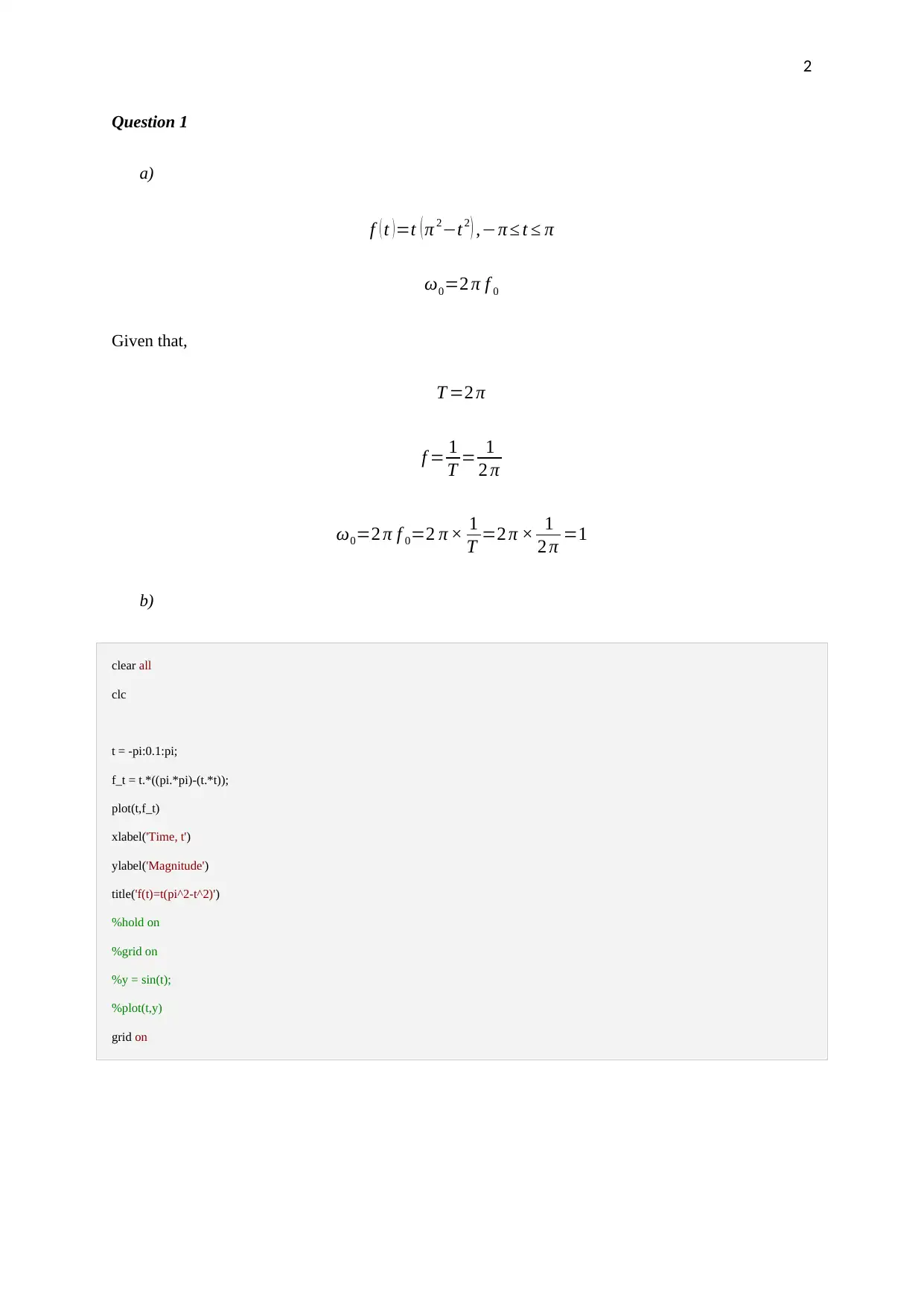
f ( t )=t ( π 2−t2 ) ,−π ≤ t ≤ π
ω0=2 π f 0
Given that,
T =2 π
f = 1
T = 1
2 π
ω0=2 π f 0=2 π × 1
T =2 π × 1
2 π =1
b)
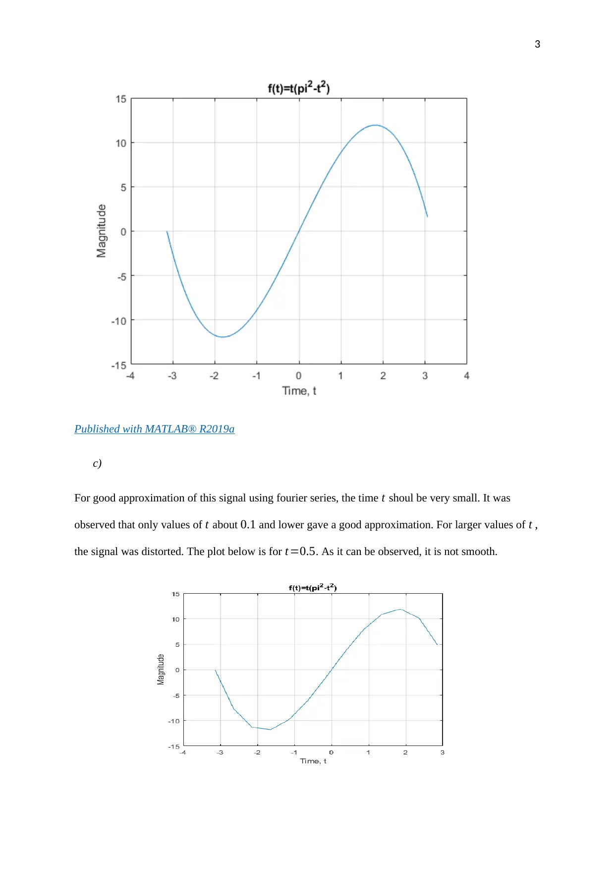
clear all
clc
t = -pi:0.1:pi;
f_t = t.*((pi.*pi)-(t.*t));
plot(t,f_t)
xlabel('Time, t')
ylabel('Magnitude')
title('f(t)=t(pi^2-t^2)')
%hold on
%grid on
%y = sin(t);
%plot(t,y)
grid on

3
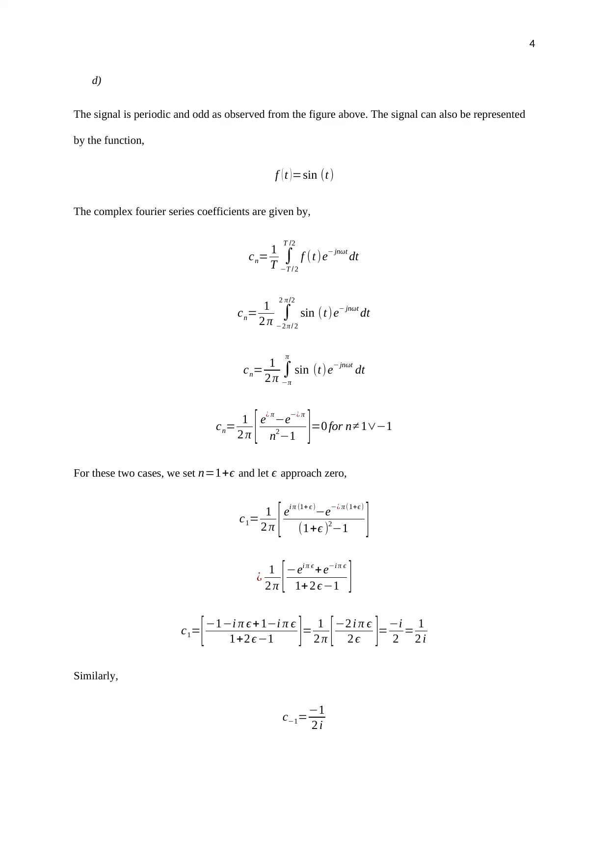
Published with MATLAB® R2019a
c)
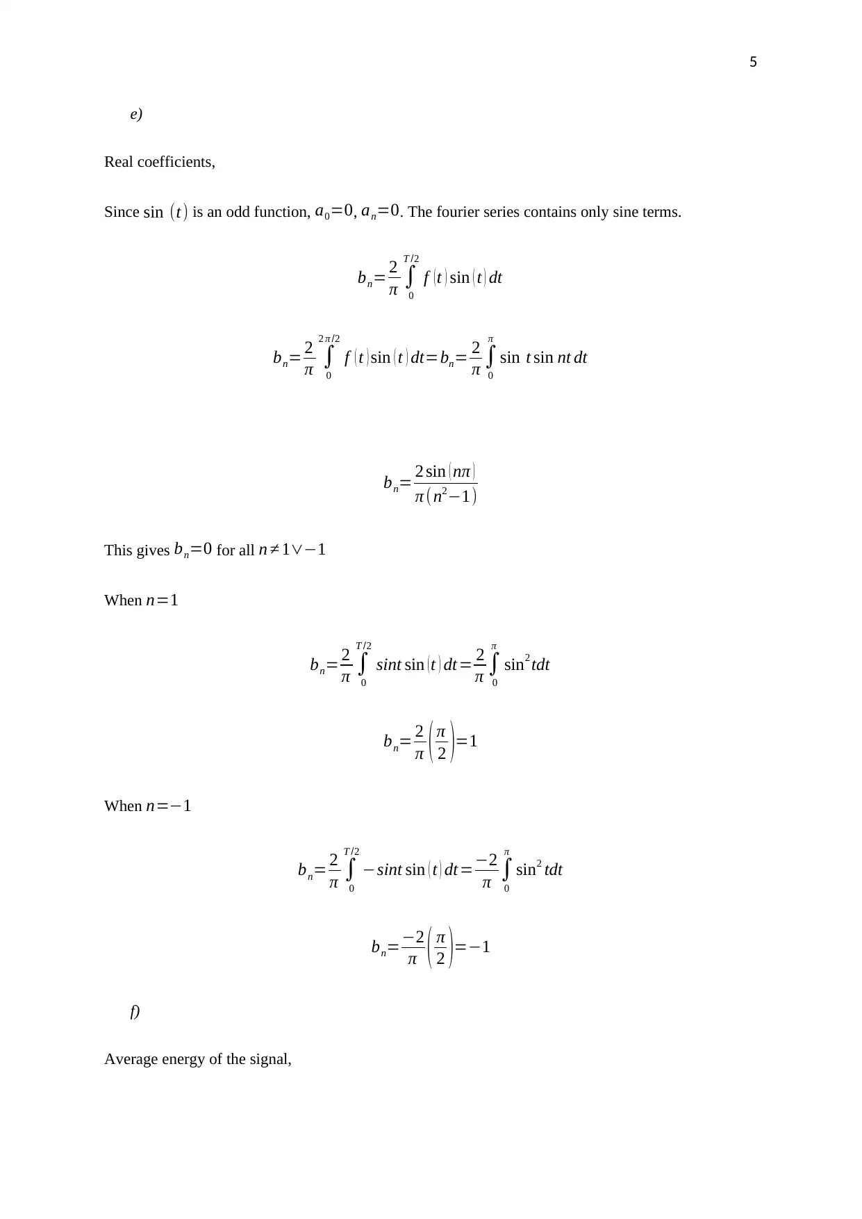
For good approximation of this signal using fourier series, the time t shoul be very small. It was
observed that only values of t about 0.1 and lower gave a good approximation. For larger values of t ,
the signal was distorted. The plot below is for t=0.5. As it can be observed, it is not smooth.

4
d)
The signal is periodic and odd as observed from the figure above. The signal can also be represented
by the function,
f ( t ) =sin (t)
The complex fourier series coefficients are given by,
cn= 1
T ∫
−T / 2
T /2
f (t )e− jnωt dt
cn= 1
2 π ∫
−2 π / 2
2 π /2
sin (t) e− jnωt dt
cn= 1
2 π ∫
−π
π
sin (t) e− jnωt dt
cn= 1
2 π [ e¿ π −e−¿ π
n2−1 ]=0 for n≠ 1∨−1
For these two cases, we set n=1+ϵ and let ϵ approach zero,
c1= 1
2 π [ ei π (1+ ϵ )−e−¿ π (1+ϵ )
(1+ϵ )2−1 ]
¿ 1
2 π [ −ei π ϵ + e−i π ϵ
1+ 2 ϵ−1 ]
c1= [ −1−i π ϵ + 1−i π ϵ
1+2 ϵ−1 ] = 1
2 π [ −2 i π ϵ
2 ϵ ]=−i
2 = 1
2 i
Similarly,
c−1=−1
2 i

5
e)
Real coefficients,
Since sin (t) is an odd function, a0=0, an=0. The fourier series contains only sine terms.
bn= 2
π ∫
0
T /2
f ( t ) sin ( t ) dt
bn= 2
π ∫
0
2 π /2
f ( t ) sin ( t ) dt=bn= 2
π ∫
0
π
sin t sin nt dt
bn= 2 sin ( nπ )
π (n2−1)
This gives bn=0 for all n ≠ 1∨−1
When n=1
bn= 2
π ∫
0
T /2
sint sin (t ) dt = 2
π ∫
0
π
sin2 tdt
bn= 2
π ( π
2 )=1
When n=−1
bn= 2
π ∫
0
T /2
−sint sin ( t ) dt =−2
π ∫
0
π
sin2 tdt
bn=−2
π ( π
2 )=−1
f)
Average energy of the signal,

6
Eav= 1
T ∫
−T / 2
T /2
¿ f ( t ) ∨¿2 dt ¿
¿ 1
2 π ∫
−π
π
¿ sint ∨¿2 dt ¿
¿ 1
2 π ∫
−π
π
¿ sint ∨¿2 dt =∫
−π
0
(−sint )2 dt+∫
0
π
sin2 tdt ¿
But,
∫
−π
0
(−sint )2 dt = π
2 =∫
0
π
sin2 tdt
Therefore,
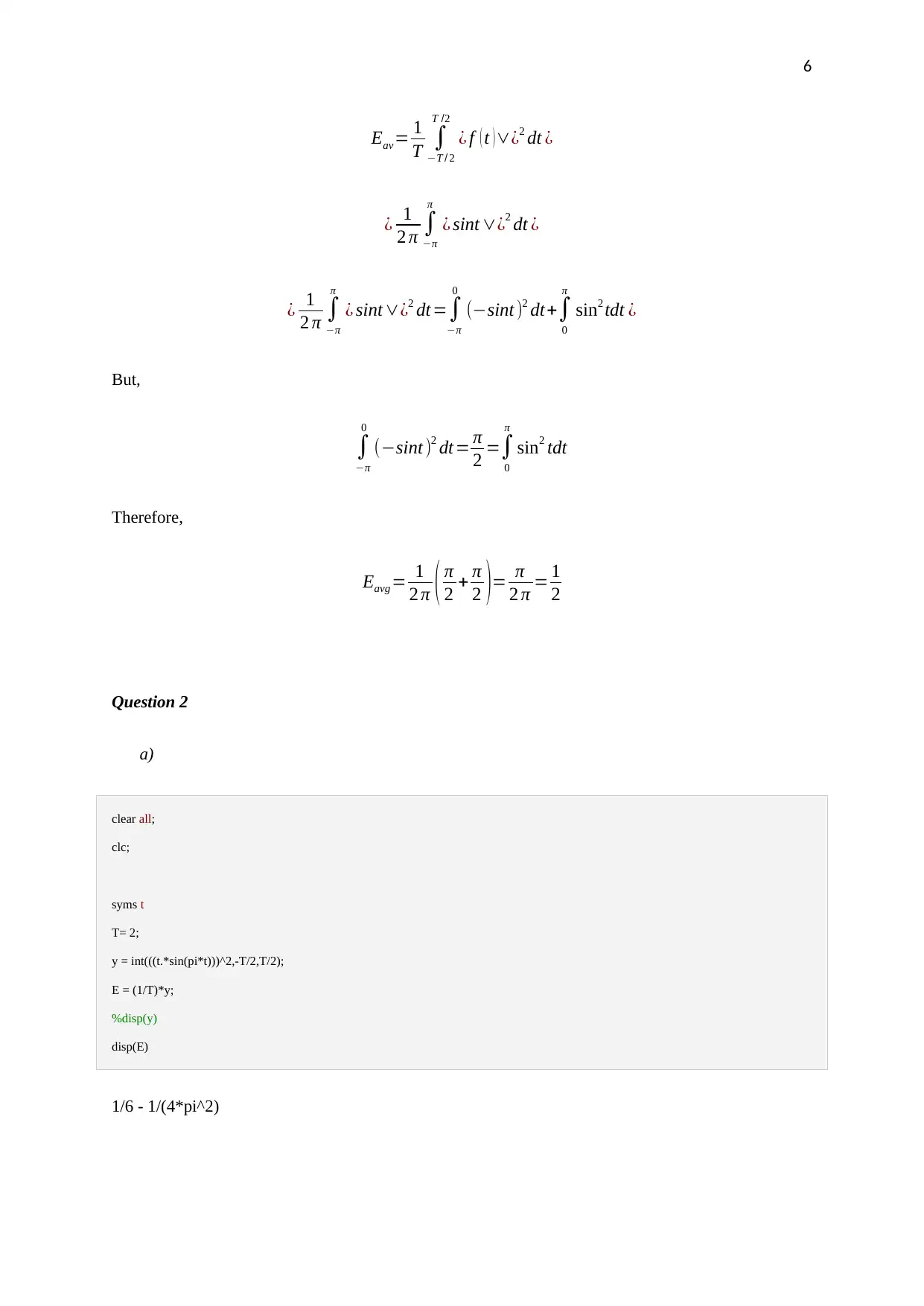
Eavg = 1
2 π ( π
2 + π
2 )= π
2 π = 1
2
Question 2
a)
clear all;
clc;
syms t
T= 2;
y = int(((t.*sin(pi*t)))^2,-T/2,T/2);
E = (1/T)*y;
%disp(y)
disp(E)
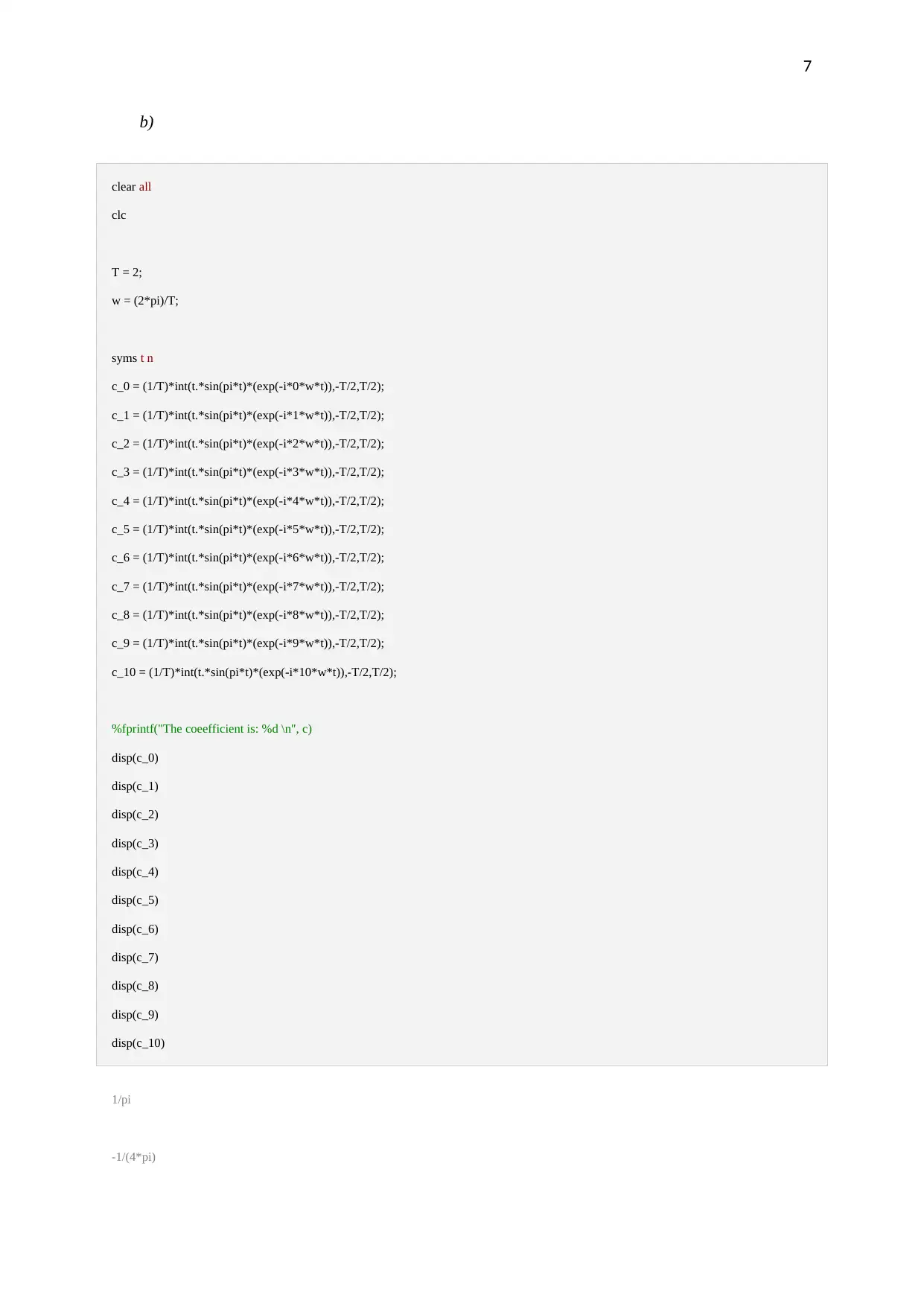
1/6 - 1/(4*pi^2)

7
b)
clear all
clc
T = 2;
w = (2*pi)/T;
syms t n
c_0 = (1/T)*int(t.*sin(pi*t)*(exp(-i*0*w*t)),-T/2,T/2);
c_1 = (1/T)*int(t.*sin(pi*t)*(exp(-i*1*w*t)),-T/2,T/2);
c_2 = (1/T)*int(t.*sin(pi*t)*(exp(-i*2*w*t)),-T/2,T/2);
c_3 = (1/T)*int(t.*sin(pi*t)*(exp(-i*3*w*t)),-T/2,T/2);
c_4 = (1/T)*int(t.*sin(pi*t)*(exp(-i*4*w*t)),-T/2,T/2);
c_5 = (1/T)*int(t.*sin(pi*t)*(exp(-i*5*w*t)),-T/2,T/2);
c_6 = (1/T)*int(t.*sin(pi*t)*(exp(-i*6*w*t)),-T/2,T/2);
c_7 = (1/T)*int(t.*sin(pi*t)*(exp(-i*7*w*t)),-T/2,T/2);
c_8 = (1/T)*int(t.*sin(pi*t)*(exp(-i*8*w*t)),-T/2,T/2);
c_9 = (1/T)*int(t.*sin(pi*t)*(exp(-i*9*w*t)),-T/2,T/2);
c_10 = (1/T)*int(t.*sin(pi*t)*(exp(-i*10*w*t)),-T/2,T/2);
%fprintf("The coeefficient is: %d \n", c)
disp(c_0)
disp(c_1)
disp(c_2)
disp(c_3)
disp(c_4)
disp(c_5)
disp(c_6)
disp(c_7)
disp(c_8)
disp(c_9)
disp(c_10)
1/pi
-1/(4*pi)

8
-1/(3*pi)
1/(8*pi)
-1/(15*pi)
1/(24*pi)
-1/(35*pi)
1/(48*pi)
-1/(63*pi)
1/(80*pi)
-1/(99*pi)
c)
clear all;
clc;
T = 2;
w = (2*pi)/T;
t = -2:0.01:2;
f_t = t.*sin(pi*t);
syms n
s_0 = symsum(exp(i*n*w*t),n,-10,10);
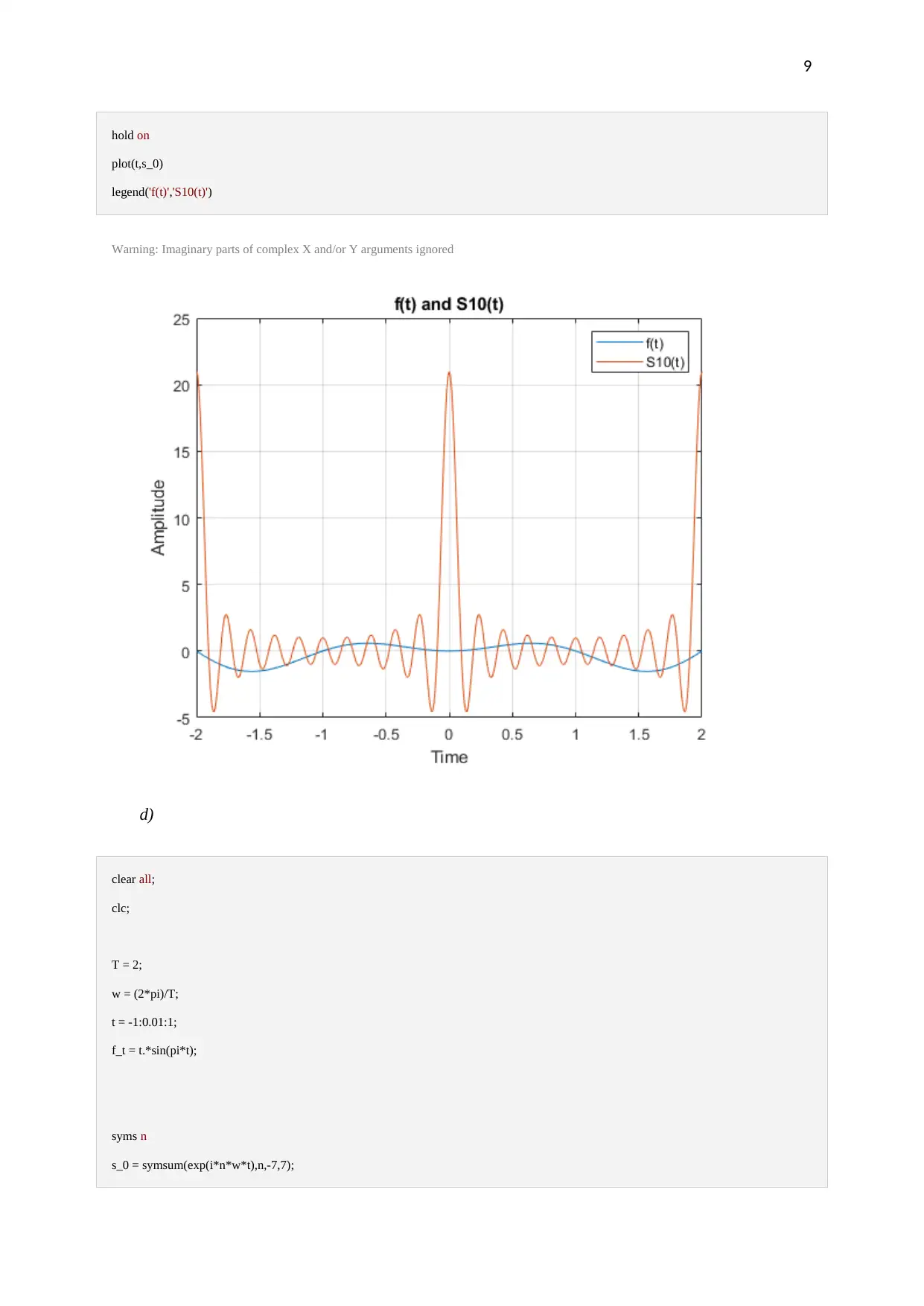
plot(t,f_t)
xlabel('Time')
ylabel('Amplitude')
title('f(t) and S10(t)')
grid on

9
hold on
plot(t,s_0)
legend('f(t)','S10(t)')
Warning: Imaginary parts of complex X and/or Y arguments ignored
d)
clear all;
clc;
T = 2;
w = (2*pi)/T;
t = -1:0.01:1;
f_t = t.*sin(pi*t);
syms n
s_0 = symsum(exp(i*n*w*t),n,-7,7);

10
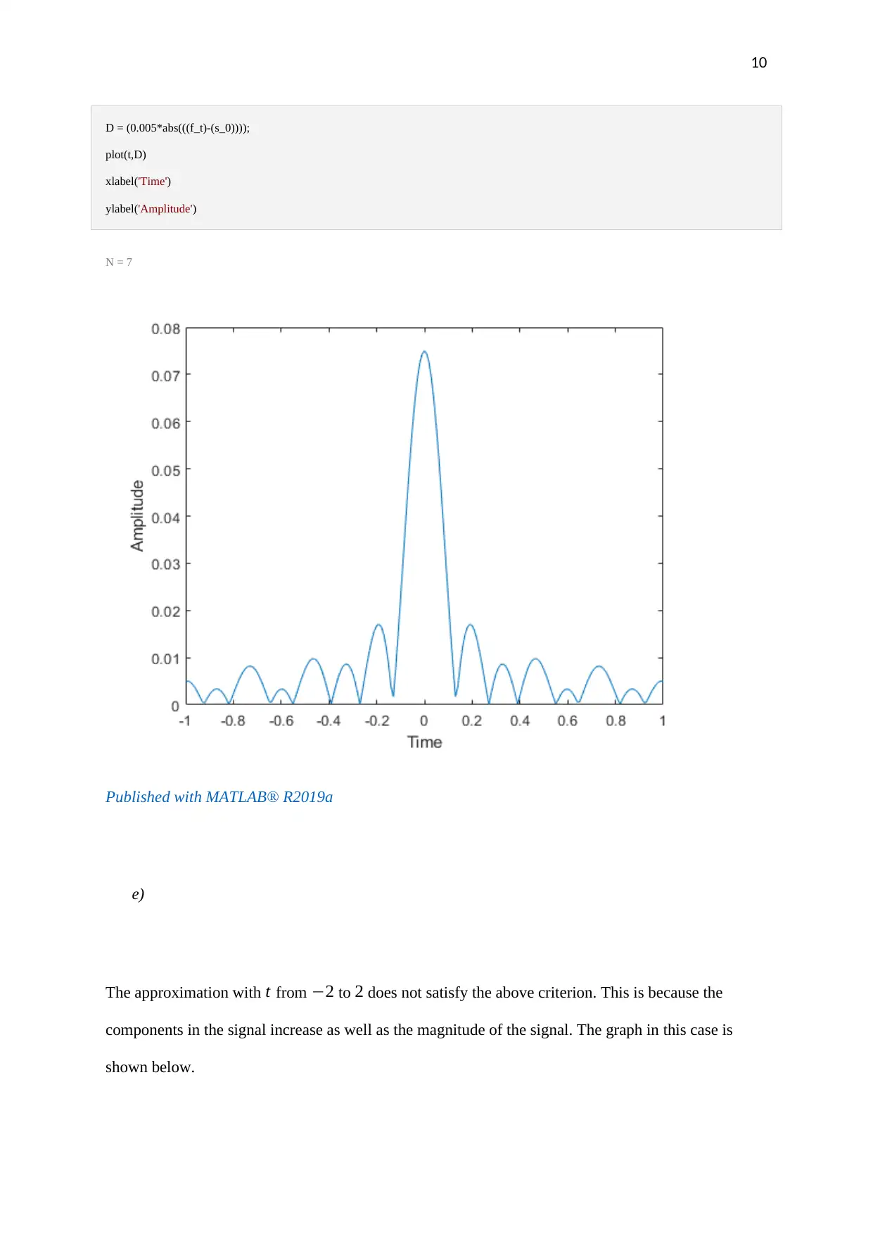
D = (0.005*abs(((f_t)-(s_0))));
plot(t,D)
xlabel('Time')
ylabel('Amplitude')
N = 7
Published with MATLAB® R2019a
e)
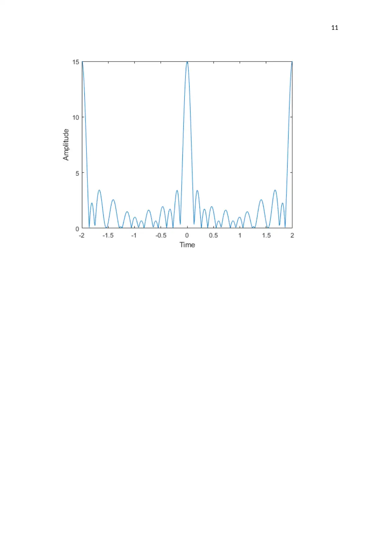
The approximation with t from −2 to 2 does not satisfy the above criterion. This is because the
components in the signal increase as well as the magnitude of the signal. The graph in this case is
shown below.

11