Regression Analysis of Factors Influencing McDonald's Stock Prices
VerifiedAdded on 2020/05/28
|12
|1772
|254
AI Summary
This research focuses on predicting changes in McDonald's stock prices using a dataset that includes variables like wheat production and West Texas oil prices. Regression analysis was employed to examine how these factors affect stock prices, revealing a significant relationship between input and output variables as evidenced by an R-squared value of 0.1712. This indicates that about 17.12% of the variance in McDonald's future stock price changes can be predicted using this model. The study also identifies key interaction terms with substantial coefficients, such as Year_x_Wheat and MCD_x_West_Texas, suggesting potential seasonal effects and cost implications due to oil prices on McDonald’s financial performance. Additionally, confidence intervals were used for predictions, which indicated some discrepancies between actual and projected values, likely attributed to the model's limited R-squared value. The study concludes by noting that while the model provides some predictive capability, its accuracy could be enhanced with a higher R-squared value.

Running head: DATA ANALYSIS
Data Analysis
Name of the Student:
Name of the University:
Author’s Note:
Data Analysis
Name of the Student:
Name of the University:
Author’s Note:
Paraphrase This Document
Need a fresh take? Get an instant paraphrase of this document with our AI Paraphraser

1
DATA ANALYSIS
Executive Summary
The report analysis stock market data from DEC 2014 to DEC 2016 on different commodities
and thus predict the future changes in the prices of McDonalds. McDonalds is one of the largest
fast food restaurant chain in the world. They are famous for hamburgers, chicken recipes and
desserts. The restaurants offer both drive through as well as counter services for its customers.
The present examination was done by analysing daily stocks data. Multiple regression analysis is
used to examine the correlation between the stock prices of McDonalds and change in prices of
other stocks. The analysis of the future prices of McDonalds is done through adjusted R2,
Analysis of Variance (ANOVA), residual analysis and Variance Inflation Factor (VIF).
2
DATA ANALYSIS
Table of Contents
Description of the data.....................................................................................................................3
Variance Inflation Factor.................................................................................................................3
Residual Analysis............................................................................................................................3
Analysis of Variance........................................................................................................................5
Coefficient of Determination R2......................................................................................................5
Hypothesis tests for the inputs.........................................................................................................6
Coefficients......................................................................................................................................6
Prediction of Tomorrow’s Share Prices...........................................................................................7
Conclusion.......................................................................................................................................8
References........................................................................................................................................9
Appendix........................................................................................................................................10
VIF.................................................................................................................................................10
⊘ This is a preview!⊘
Do you want full access?
Subscribe today to unlock all pages.
Trusted by 1+ million students worldwide
3
DATA ANALYSIS
Description of the data
The data presents the stock prices from 8th Dec 2014 to 1st Dec 2016 (383 days). In
addition, the data contains inputs from 8 independent variables and one dependent variable
(future prices of McDonalds). For each of the 383 days the change in prices of the assets
measured are:
Copper
Aluminium
West Texas Intermediate Oil
The Baltic Dry Index
The Standard and Poors 500 Index of stock prices (the S&P500)
Also McDonalds future prices
Most of the variables used to predict the future change are interaction variables. Moreover,
some of the variables have a suffix “vel” or “acc.” “vel” followed by a number refers to the
change in price in the number of days. “acc” refers to the change in velocity.
Thus while “copper” would have referred to the price of “copper”, “copper_acc1” would indicate
how the price of copper accelerates (decelerates) over a period of 2 days.
Similarly “MCD_vel2” means the change in price of McDonalds going back one day.
Variance Inflation Factor
Variance inflation factor (VIF) is used to assess multi-collinearity in a data-set. Multi-
collinearity refers to the phenomenon of correlation between two or more variables in
multi-regression. In the situation that Multi-collinearity exists in a model, with the
addition of more predictors the precision of the regression coefficient of the model
decreases.
The test for VIF showed that there is no or very low correlation between the input
variables. The VIF for each of the 8 factors was found to be ≤ 5. PhSTAT software was
used to find multi-collinearity.
Thus it can be inferred that all the 8 response variables which are used to measure the
future prices of McDonalds are independent and thus can be used in the model.
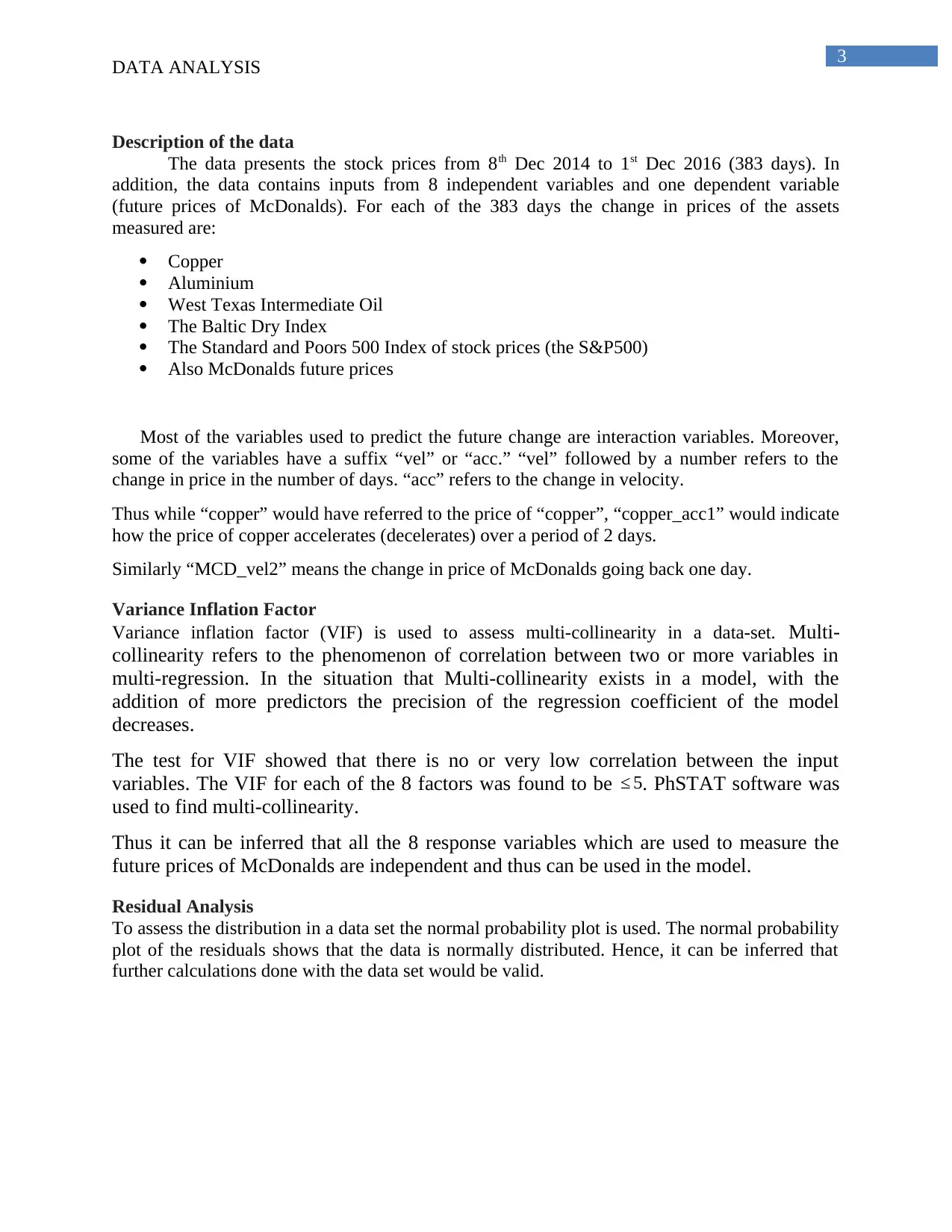
Residual Analysis
To assess the distribution in a data set the normal probability plot is used. The normal probability
plot of the residuals shows that the data is normally distributed. Hence, it can be inferred that
further calculations done with the data set would be valid.
DATA ANALYSIS
Description of the data
The data presents the stock prices from 8th Dec 2014 to 1st Dec 2016 (383 days). In
addition, the data contains inputs from 8 independent variables and one dependent variable
(future prices of McDonalds). For each of the 383 days the change in prices of the assets
measured are:
Copper
Aluminium
West Texas Intermediate Oil
The Baltic Dry Index
The Standard and Poors 500 Index of stock prices (the S&P500)
Also McDonalds future prices
Most of the variables used to predict the future change are interaction variables. Moreover,
some of the variables have a suffix “vel” or “acc.” “vel” followed by a number refers to the
change in price in the number of days. “acc” refers to the change in velocity.
Thus while “copper” would have referred to the price of “copper”, “copper_acc1” would indicate
how the price of copper accelerates (decelerates) over a period of 2 days.
Similarly “MCD_vel2” means the change in price of McDonalds going back one day.
Variance Inflation Factor
Variance inflation factor (VIF) is used to assess multi-collinearity in a data-set. Multi-
collinearity refers to the phenomenon of correlation between two or more variables in
multi-regression. In the situation that Multi-collinearity exists in a model, with the
addition of more predictors the precision of the regression coefficient of the model
decreases.
The test for VIF showed that there is no or very low correlation between the input
variables. The VIF for each of the 8 factors was found to be ≤ 5. PhSTAT software was
used to find multi-collinearity.
Thus it can be inferred that all the 8 response variables which are used to measure the
future prices of McDonalds are independent and thus can be used in the model.
Residual Analysis
To assess the distribution in a data set the normal probability plot is used. The normal probability
plot of the residuals shows that the data is normally distributed. Hence, it can be inferred that
further calculations done with the data set would be valid.
Paraphrase This Document
Need a fresh take? Get an instant paraphrase of this document with our AI Paraphraser
4
DATA ANALYSIS
-4 -3 -2 -1 0 1 2 3 4
-0.8
-0.6
-0.4
-0.2
0
0.2
0.4
0.6
0.8
Normal Probability Plot
Z Value
Residual
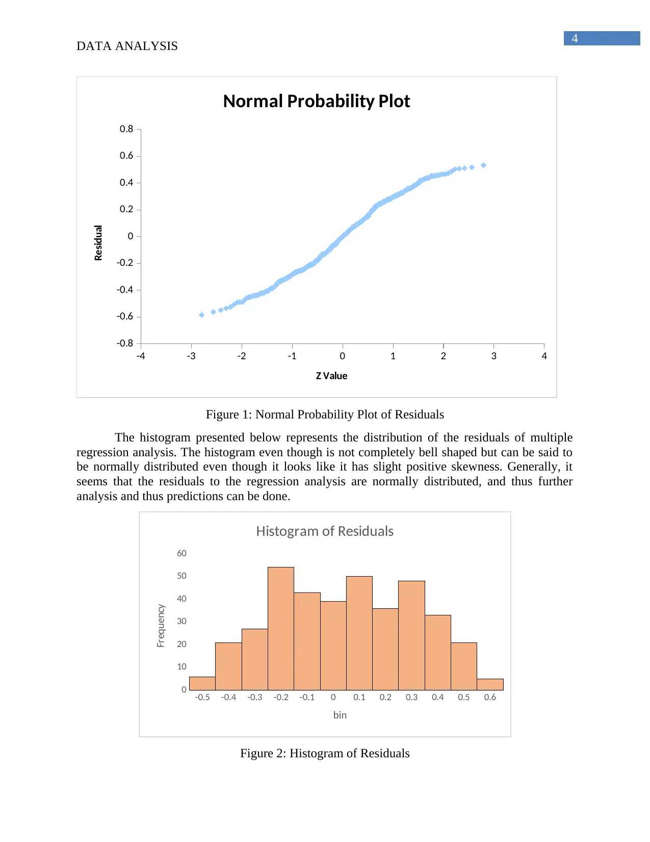
Figure 1: Normal Probability Plot of Residuals
The histogram presented below represents the distribution of the residuals of multiple
regression analysis. The histogram even though is not completely bell shaped but can be said to
be normally distributed even though it looks like it has slight positive skewness. Generally, it
seems that the residuals to the regression analysis are normally distributed, and thus further
analysis and thus predictions can be done.
-0.5 -0.4 -0.3 -0.2 -0.1 0 0.1 0.2 0.3 0.4 0.5 0.6
0
10
20
30
40
50
60
Histogram of Residuals
bin
Frequency
Figure 2: Histogram of Residuals
DATA ANALYSIS
-4 -3 -2 -1 0 1 2 3 4
-0.8
-0.6
-0.4
-0.2
0
0.2
0.4
0.6
0.8
Normal Probability Plot
Z Value
Residual
Figure 1: Normal Probability Plot of Residuals
The histogram presented below represents the distribution of the residuals of multiple
regression analysis. The histogram even though is not completely bell shaped but can be said to
be normally distributed even though it looks like it has slight positive skewness. Generally, it
seems that the residuals to the regression analysis are normally distributed, and thus further
analysis and thus predictions can be done.
-0.5 -0.4 -0.3 -0.2 -0.1 0 0.1 0.2 0.3 0.4 0.5 0.6
0
10
20
30
40
50
60
Histogram of Residuals
bin
Frequency
Figure 2: Histogram of Residuals
5
DATA ANALYSIS
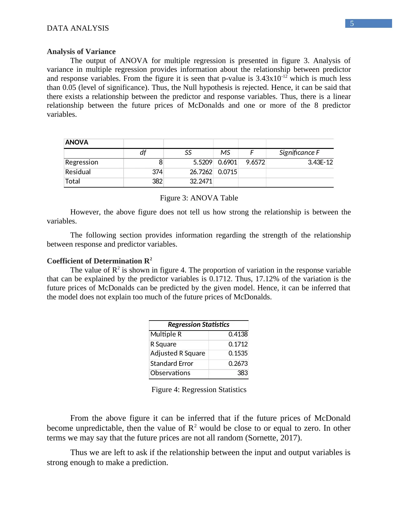
Analysis of Variance
The output of ANOVA for multiple regression is presented in figure 3. Analysis of
variance in multiple regression provides information about the relationship between predictor
and response variables. From the figure it is seen that p-value is 3.43x10⁻¹² which is much less
than 0.05 (level of significance). Thus, the Null hypothesis is rejected. Hence, it can be said that
there exists a relationship between the predictor and response variables. Thus, there is a linear
relationship between the future prices of McDonalds and one or more of the 8 predictor
variables.
ANOVA
df SS MS F Significance F
Regression 8 5.5209 0.6901 9.6572 3.43E-12
Residual 374 26.7262 0.0715
Total 382 32.2471
Figure 3: ANOVA Table
However, the above figure does not tell us how strong the relationship is between the
variables.
The following section provides information regarding the strength of the relationship
between response and predictor variables.
Coefficient of Determination R2
The value of R2 is shown in figure 4. The proportion of variation in the response variable
that can be explained by the predictor variables is 0.1712. Thus, 17.12% of the variation is the
future prices of McDonalds can be predicted by the given model. Hence, it can be inferred that
the model does not explain too much of the future prices of McDonalds.
Regression Statistics
Multiple R 0.4138
R Square 0.1712
Adjusted R Square 0.1535
Standard Error 0.2673
Observations 383
Figure 4: Regression Statistics
From the above figure it can be inferred that if the future prices of McDonald
become unpredictable, then the value of R2 would be close to or equal to zero. In other
terms we may say that the future prices are not all random (Sornette, 2017).
Thus we are left to ask if the relationship between the input and output variables is
strong enough to make a prediction.
DATA ANALYSIS
Analysis of Variance
The output of ANOVA for multiple regression is presented in figure 3. Analysis of
variance in multiple regression provides information about the relationship between predictor
and response variables. From the figure it is seen that p-value is 3.43x10⁻¹² which is much less
than 0.05 (level of significance). Thus, the Null hypothesis is rejected. Hence, it can be said that
there exists a relationship between the predictor and response variables. Thus, there is a linear
relationship between the future prices of McDonalds and one or more of the 8 predictor
variables.
ANOVA
df SS MS F Significance F
Regression 8 5.5209 0.6901 9.6572 3.43E-12
Residual 374 26.7262 0.0715
Total 382 32.2471
Figure 3: ANOVA Table
However, the above figure does not tell us how strong the relationship is between the
variables.
The following section provides information regarding the strength of the relationship
between response and predictor variables.
Coefficient of Determination R2
The value of R2 is shown in figure 4. The proportion of variation in the response variable
that can be explained by the predictor variables is 0.1712. Thus, 17.12% of the variation is the
future prices of McDonalds can be predicted by the given model. Hence, it can be inferred that
the model does not explain too much of the future prices of McDonalds.
Regression Statistics
Multiple R 0.4138
R Square 0.1712
Adjusted R Square 0.1535
Standard Error 0.2673
Observations 383
Figure 4: Regression Statistics
From the above figure it can be inferred that if the future prices of McDonald
become unpredictable, then the value of R2 would be close to or equal to zero. In other
terms we may say that the future prices are not all random (Sornette, 2017).
Thus we are left to ask if the relationship between the input and output variables is
strong enough to make a prediction.
⊘ This is a preview!⊘
Do you want full access?
Subscribe today to unlock all pages.
Trusted by 1+ million students worldwide
6
DATA ANALYSIS
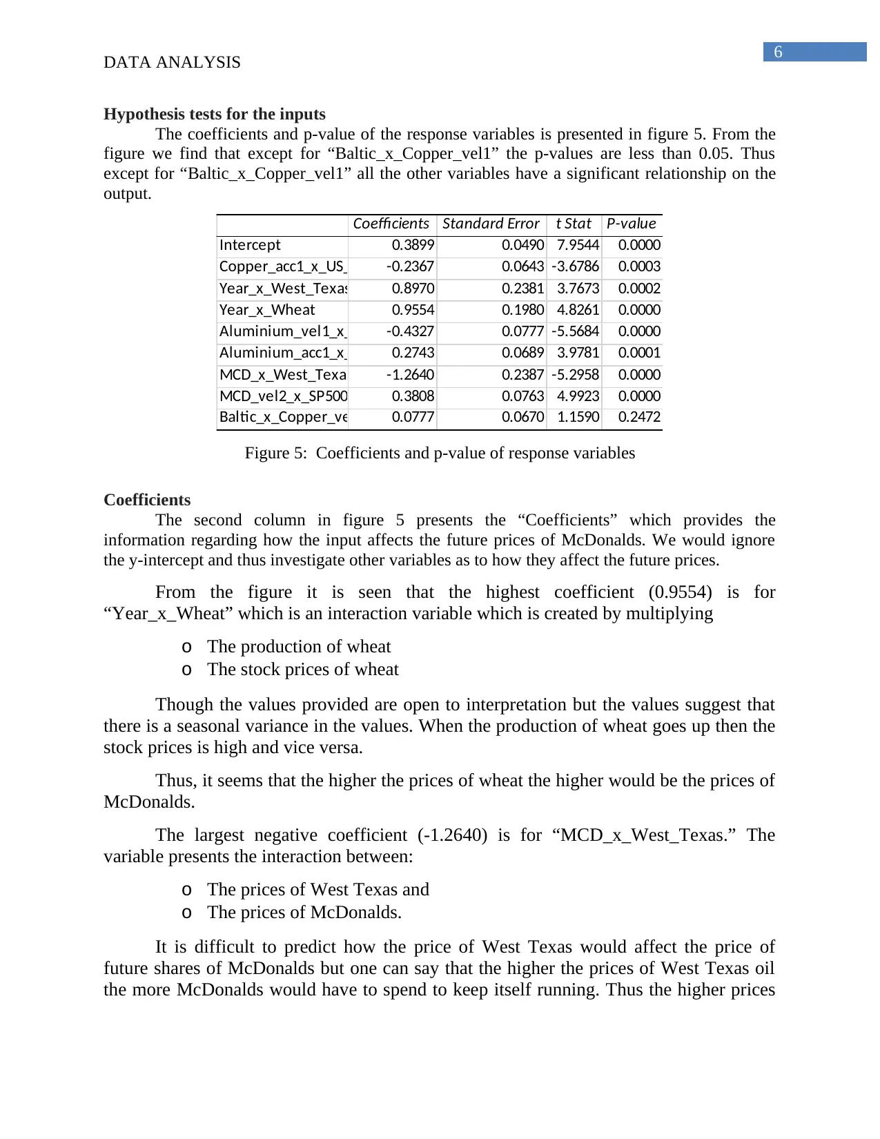
Hypothesis tests for the inputs
The coefficients and p-value of the response variables is presented in figure 5. From the
figure we find that except for “Baltic_x_Copper_vel1” the p-values are less than 0.05. Thus
except for “Baltic_x_Copper_vel1” all the other variables have a significant relationship on the
output.
Coefficients Standard Error t Stat P-value
Intercept 0.3899 0.0490 7.9544 0.0000
Copper_acc1_x_US_Realty_vel1-0.2367 0.0643 -3.6786 0.0003
Year_x_West_Texas 0.8970 0.2381 3.7673 0.0002
Year_x_Wheat 0.9554 0.1980 4.8261 0.0000
Aluminium_vel1_x_MCD_vel2-0.4327 0.0777 -5.5684 0.0000
Aluminium_acc1_x_Gold 0.2743 0.0689 3.9781 0.0001
MCD_x_West_Texas -1.2640 0.2387 -5.2958 0.0000
MCD_vel2_x_SP500_acc1 0.3808 0.0763 4.9923 0.0000
Baltic_x_Copper_vel1 0.0777 0.0670 1.1590 0.2472
Figure 5: Coefficients and p-value of response variables
Coefficients
The second column in figure 5 presents the “Coefficients” which provides the
information regarding how the input affects the future prices of McDonalds. We would ignore
the y-intercept and thus investigate other variables as to how they affect the future prices.
From the figure it is seen that the highest coefficient (0.9554) is for
“Year_x_Wheat” which is an interaction variable which is created by multiplying
o The production of wheat
o The stock prices of wheat
Though the values provided are open to interpretation but the values suggest that
there is a seasonal variance in the values. When the production of wheat goes up then the
stock prices is high and vice versa.
Thus, it seems that the higher the prices of wheat the higher would be the prices of
McDonalds.
The largest negative coefficient (-1.2640) is for “MCD_x_West_Texas.” The
variable presents the interaction between:
o The prices of West Texas and
o The prices of McDonalds.
It is difficult to predict how the price of West Texas would affect the price of
future shares of McDonalds but one can say that the higher the prices of West Texas oil
the more McDonalds would have to spend to keep itself running. Thus the higher prices
DATA ANALYSIS
Hypothesis tests for the inputs
The coefficients and p-value of the response variables is presented in figure 5. From the
figure we find that except for “Baltic_x_Copper_vel1” the p-values are less than 0.05. Thus
except for “Baltic_x_Copper_vel1” all the other variables have a significant relationship on the
output.
Coefficients Standard Error t Stat P-value
Intercept 0.3899 0.0490 7.9544 0.0000
Copper_acc1_x_US_Realty_vel1-0.2367 0.0643 -3.6786 0.0003
Year_x_West_Texas 0.8970 0.2381 3.7673 0.0002
Year_x_Wheat 0.9554 0.1980 4.8261 0.0000
Aluminium_vel1_x_MCD_vel2-0.4327 0.0777 -5.5684 0.0000
Aluminium_acc1_x_Gold 0.2743 0.0689 3.9781 0.0001
MCD_x_West_Texas -1.2640 0.2387 -5.2958 0.0000
MCD_vel2_x_SP500_acc1 0.3808 0.0763 4.9923 0.0000
Baltic_x_Copper_vel1 0.0777 0.0670 1.1590 0.2472
Figure 5: Coefficients and p-value of response variables
Coefficients
The second column in figure 5 presents the “Coefficients” which provides the
information regarding how the input affects the future prices of McDonalds. We would ignore
the y-intercept and thus investigate other variables as to how they affect the future prices.
From the figure it is seen that the highest coefficient (0.9554) is for
“Year_x_Wheat” which is an interaction variable which is created by multiplying
o The production of wheat
o The stock prices of wheat
Though the values provided are open to interpretation but the values suggest that
there is a seasonal variance in the values. When the production of wheat goes up then the
stock prices is high and vice versa.
Thus, it seems that the higher the prices of wheat the higher would be the prices of
McDonalds.
The largest negative coefficient (-1.2640) is for “MCD_x_West_Texas.” The
variable presents the interaction between:
o The prices of West Texas and
o The prices of McDonalds.
It is difficult to predict how the price of West Texas would affect the price of
future shares of McDonalds but one can say that the higher the prices of West Texas oil
the more McDonalds would have to spend to keep itself running. Thus the higher prices
Paraphrase This Document
Need a fresh take? Get an instant paraphrase of this document with our AI Paraphraser
7
DATA ANALYSIS
of West Texas would influence the stock prices of McDonalds. However, this explanation
is subject to interpretation.
Since, neither of the coefficients of the input variables are close to zero, hence it
can be said that the input variables have a relationship with the output variable. Thus,
there is no need to delete any input variable.
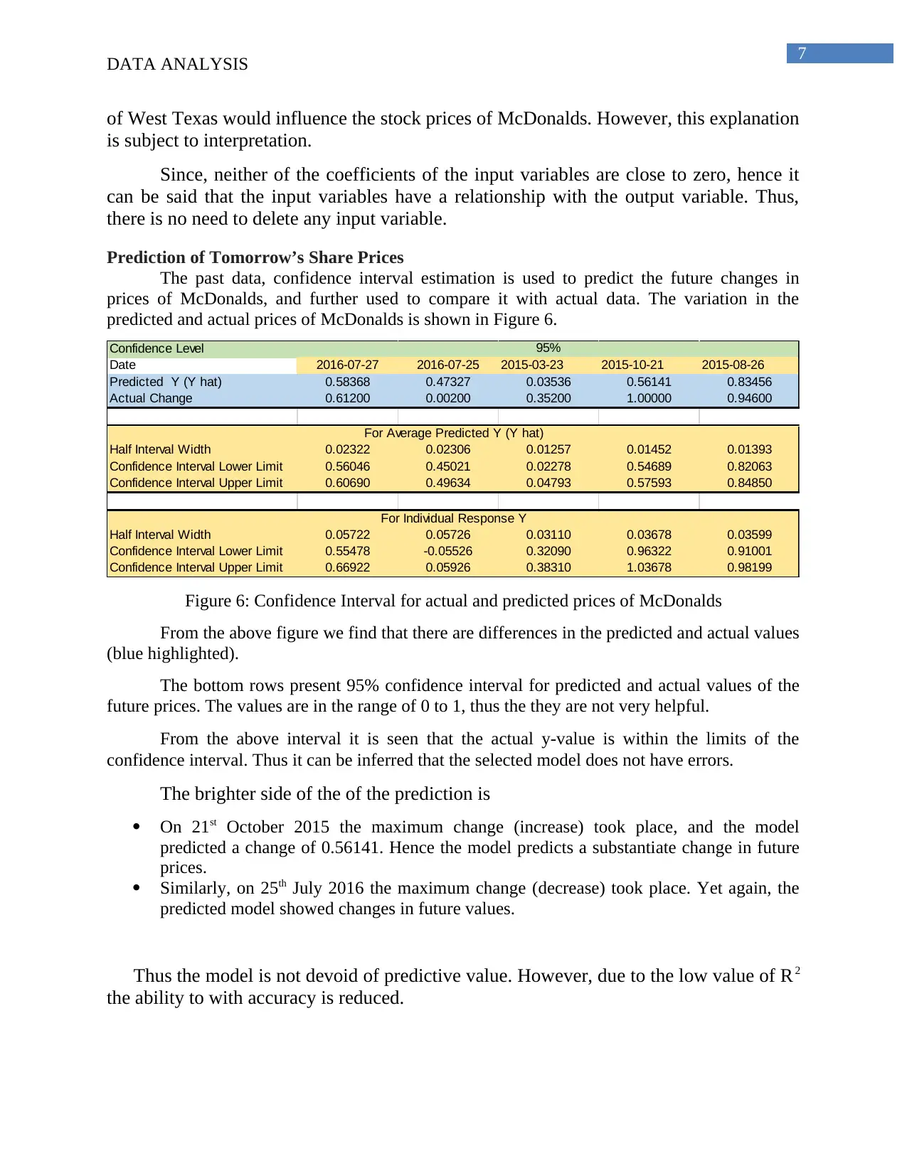
Prediction of Tomorrow’s Share Prices
The past data, confidence interval estimation is used to predict the future changes in
prices of McDonalds, and further used to compare it with actual data. The variation in the
predicted and actual prices of McDonalds is shown in Figure 6.
Confidence Level
Date 2016-07-27 2016-07-25 2015-03-23 2015-10-21 2015-08-26
Predicted Y (Y hat) 0.58368 0.47327 0.03536 0.56141 0.83456
Actual Change 0.61200 0.00200 0.35200 1.00000 0.94600
Half Interval Width 0.02322 0.02306 0.01257 0.01452 0.01393
Confidence Interval Lower Limit 0.56046 0.45021 0.02278 0.54689 0.82063
Confidence Interval Upper Limit 0.60690 0.49634 0.04793 0.57593 0.84850
Half Interval Width 0.05722 0.05726 0.03110 0.03678 0.03599
Confidence Interval Lower Limit 0.55478 -0.05526 0.32090 0.96322 0.91001
Confidence Interval Upper Limit 0.66922 0.05926 0.38310 1.03678 0.98199
95%
For Individual Response Y
For Average Predicted Y (Y hat)
Figure 6: Confidence Interval for actual and predicted prices of McDonalds
From the above figure we find that there are differences in the predicted and actual values
(blue highlighted).
The bottom rows present 95% confidence interval for predicted and actual values of the
future prices. The values are in the range of 0 to 1, thus the they are not very helpful.
From the above interval it is seen that the actual y-value is within the limits of the
confidence interval. Thus it can be inferred that the selected model does not have errors.
The brighter side of the of the prediction is
On 21st October 2015 the maximum change (increase) took place, and the model
predicted a change of 0.56141. Hence the model predicts a substantiate change in future
prices.
Similarly, on 25th July 2016 the maximum change (decrease) took place. Yet again, the
predicted model showed changes in future values.
Thus the model is not devoid of predictive value. However, due to the low value of R2
the ability to with accuracy is reduced.
DATA ANALYSIS
of West Texas would influence the stock prices of McDonalds. However, this explanation
is subject to interpretation.
Since, neither of the coefficients of the input variables are close to zero, hence it
can be said that the input variables have a relationship with the output variable. Thus,
there is no need to delete any input variable.
Prediction of Tomorrow’s Share Prices
The past data, confidence interval estimation is used to predict the future changes in
prices of McDonalds, and further used to compare it with actual data. The variation in the
predicted and actual prices of McDonalds is shown in Figure 6.
Confidence Level
Date 2016-07-27 2016-07-25 2015-03-23 2015-10-21 2015-08-26
Predicted Y (Y hat) 0.58368 0.47327 0.03536 0.56141 0.83456
Actual Change 0.61200 0.00200 0.35200 1.00000 0.94600
Half Interval Width 0.02322 0.02306 0.01257 0.01452 0.01393
Confidence Interval Lower Limit 0.56046 0.45021 0.02278 0.54689 0.82063
Confidence Interval Upper Limit 0.60690 0.49634 0.04793 0.57593 0.84850
Half Interval Width 0.05722 0.05726 0.03110 0.03678 0.03599
Confidence Interval Lower Limit 0.55478 -0.05526 0.32090 0.96322 0.91001
Confidence Interval Upper Limit 0.66922 0.05926 0.38310 1.03678 0.98199
95%
For Individual Response Y
For Average Predicted Y (Y hat)
Figure 6: Confidence Interval for actual and predicted prices of McDonalds
From the above figure we find that there are differences in the predicted and actual values
(blue highlighted).
The bottom rows present 95% confidence interval for predicted and actual values of the
future prices. The values are in the range of 0 to 1, thus the they are not very helpful.
From the above interval it is seen that the actual y-value is within the limits of the
confidence interval. Thus it can be inferred that the selected model does not have errors.
The brighter side of the of the prediction is
On 21st October 2015 the maximum change (increase) took place, and the model
predicted a change of 0.56141. Hence the model predicts a substantiate change in future
prices.
Similarly, on 25th July 2016 the maximum change (decrease) took place. Yet again, the
predicted model showed changes in future values.
Thus the model is not devoid of predictive value. However, due to the low value of R2
the ability to with accuracy is reduced.
8
DATA ANALYSIS
Conclusion
The data set is used to predict the future changes in the stock prices of McDonalds. From
the VIF test it is seen that there is no correlation between the independent variables. The
normal probability plot and Histogram shows that the residual of the multiple regression
is normally distributed. From the multiple regression it is found that the value of R2 is
0.1712. Thus, it can be said that 17.12% changes in the future stock prices of McDonalds
can be predicted by the following model. Moreover, from the ANOVA table it is seen
that a significant relationship exists between the input and out variables.
Figure 6 presents the predicted changes in future prices of McDonalds. There exist
differences in predicted and actual prices. The difference in values is due to the fact that
the value of R2 can predict only 17.12% change. The difference between predicted and
actual could plausibly be reduced with a higher value of R2.
⊘ This is a preview!⊘
Do you want full access?
Subscribe today to unlock all pages.
Trusted by 1+ million students worldwide

9
DATA ANALYSIS
References
Sornette, D. (2017). Why stock markets crash: critical events in complex financial systems.
Princeton University Press.
DATA ANALYSIS
References
Sornette, D. (2017). Why stock markets crash: critical events in complex financial systems.
Princeton University Press.
Paraphrase This Document
Need a fresh take? Get an instant paraphrase of this document with our AI Paraphraser

10
DATA ANALYSIS
Appendix
VIF
Regression Analysis
Copper_acc1_x_US_Realty_vel1 and all other X
Regression Statistics
Multiple R 0.4288
R Square 0.1839
Adjusted R Square 0.1687
Standard Error 0.2145
Observations 383
VIF 1.2253
Regression Analysis
Year_x_West_Texas and all other X
Regression Statistics
Multiple R 0.8306
R Square 0.6898
Adjusted R Square 0.6840
Standard Error 0.0580
Observations 383
VIF 3.2241
Regression Analysis
Year_x_Wheat and all other X
Regression Statistics
Multiple R 0.5647
R Square 0.3189
Adjusted R Square 0.3062
Standard Error 0.0697
Observations 383
VIF 1.4682
Regression Analysis
Aluminium_vel1_x_MCD_vel2 and all other X
Regression Statistics
Multiple R 0.5753
R Square 0.3310
Adjusted R Square 0.3185
Standard Error 0.1776
Observations 383
VIF 1.4948
Regression Analysis
Aluminium_acc1_x_Gold and all other X
Regression Statistics
Multiple R 0.4918
R Square 0.2419
Adjusted R Square 0.2277
Standard Error 0.2002
Observations 383
VIF 1.3190
Regression Analysis
MCD_x_West_Texas and all other X
Regression Statistics
Multiple R 0.8429
R Square 0.7106
Adjusted R Square 0.7052
Standard Error 0.0578
Observations 383
VIF 3.4550
11
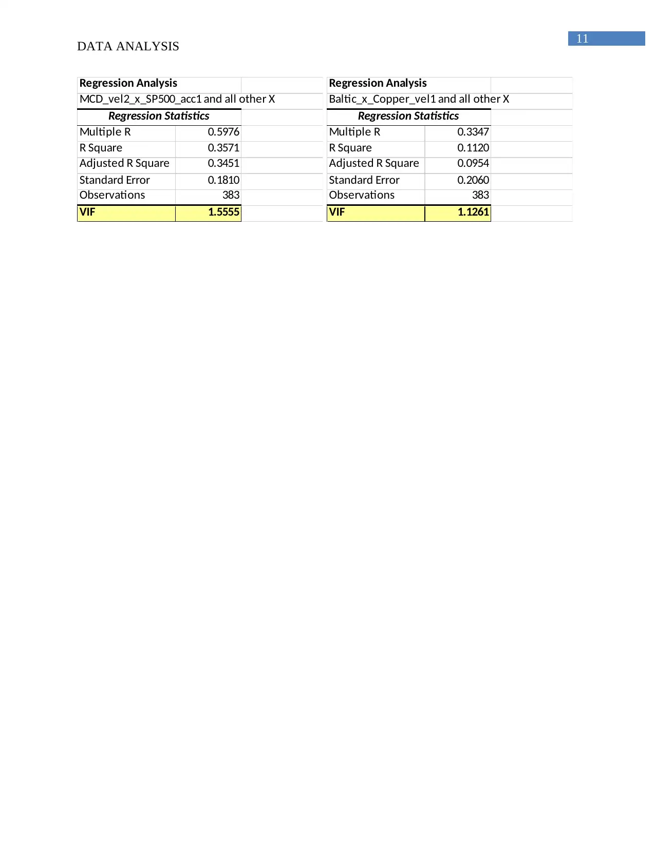
DATA ANALYSIS
Regression Analysis
MCD_vel2_x_SP500_acc1 and all other X
Regression Statistics
Multiple R 0.5976
R Square 0.3571
Adjusted R Square 0.3451
Standard Error 0.1810
Observations 383
VIF 1.5555
Regression Analysis
Baltic_x_Copper_vel1 and all other X
Regression Statistics
Multiple R 0.3347
R Square 0.1120
Adjusted R Square 0.0954
Standard Error 0.2060
Observations 383
VIF 1.1261
⊘ This is a preview!⊘
Do you want full access?
Subscribe today to unlock all pages.
Trusted by 1+ million students worldwide
1 out of 12
Related Documents


Your All-in-One AI-Powered Toolkit for Academic Success.
+13062052269
info@desklib.com
Available 24*7 on WhatsApp / Email
![[object Object]](/_next/static/media/star-bottom.7253800d.svg)
Unlock your academic potential
Copyright © 2020–2026 A2Z Services. All Rights Reserved. Developed and managed by ZUCOL.