MEC3456 Lab 07: Application of Numerical Methods in Solving ODEs

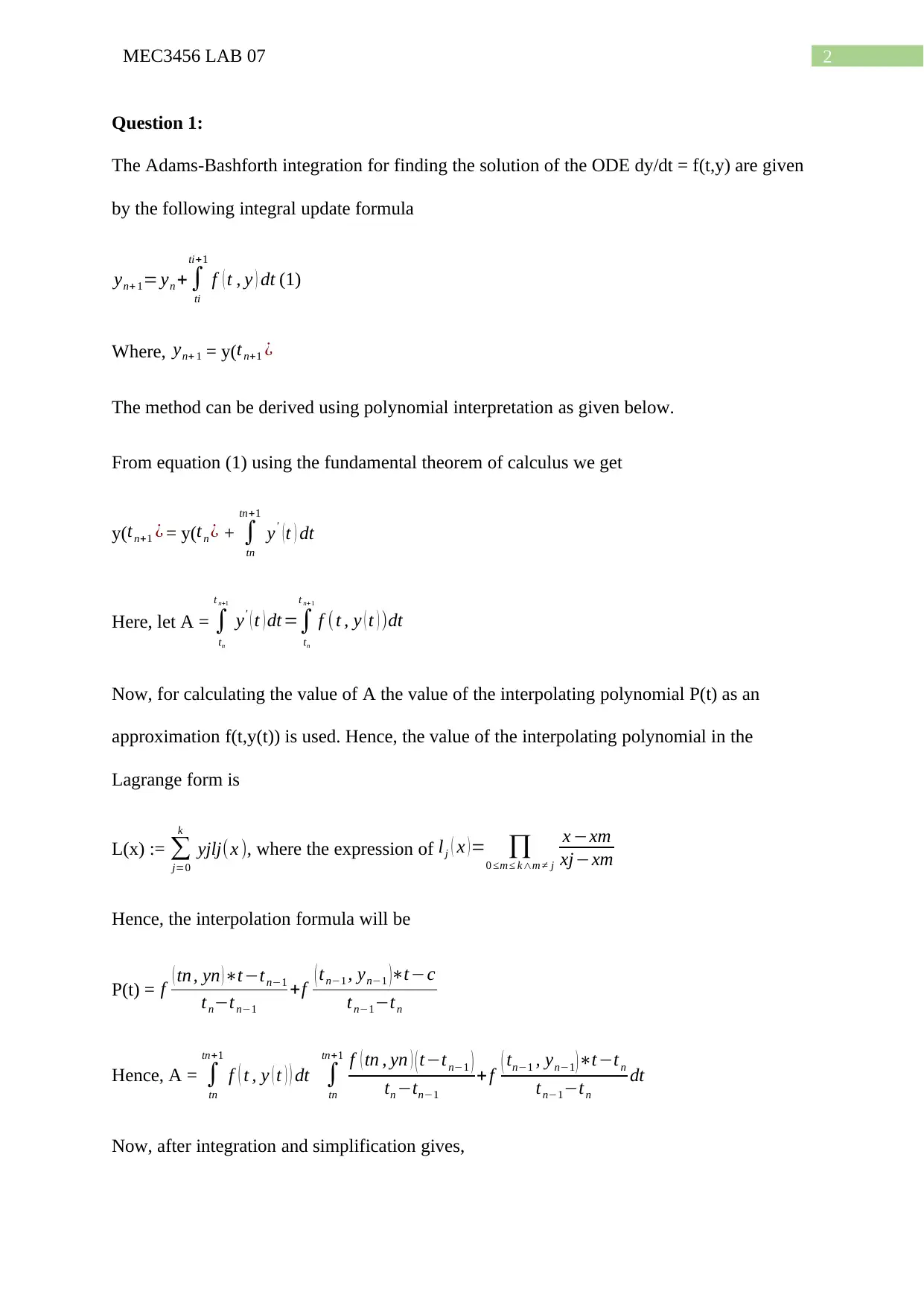
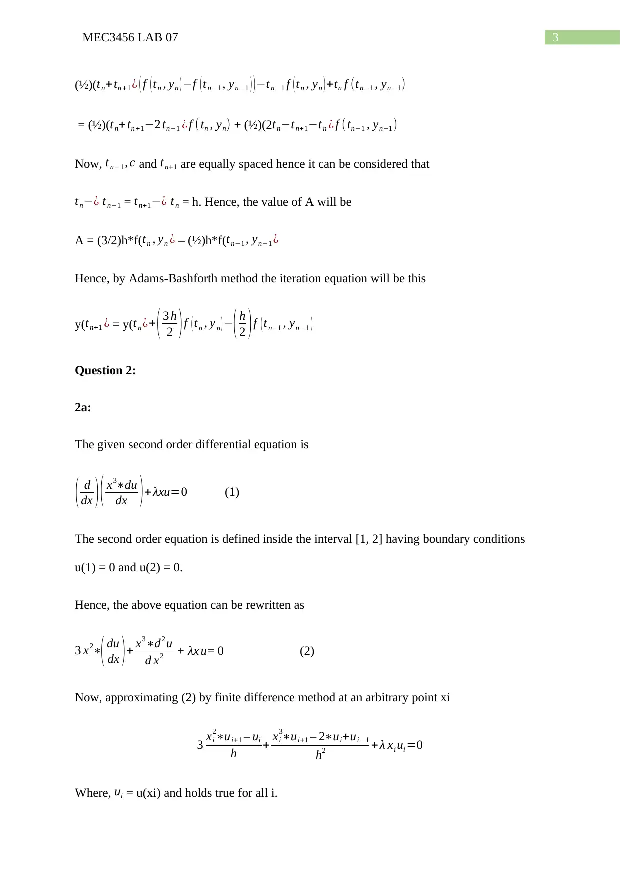
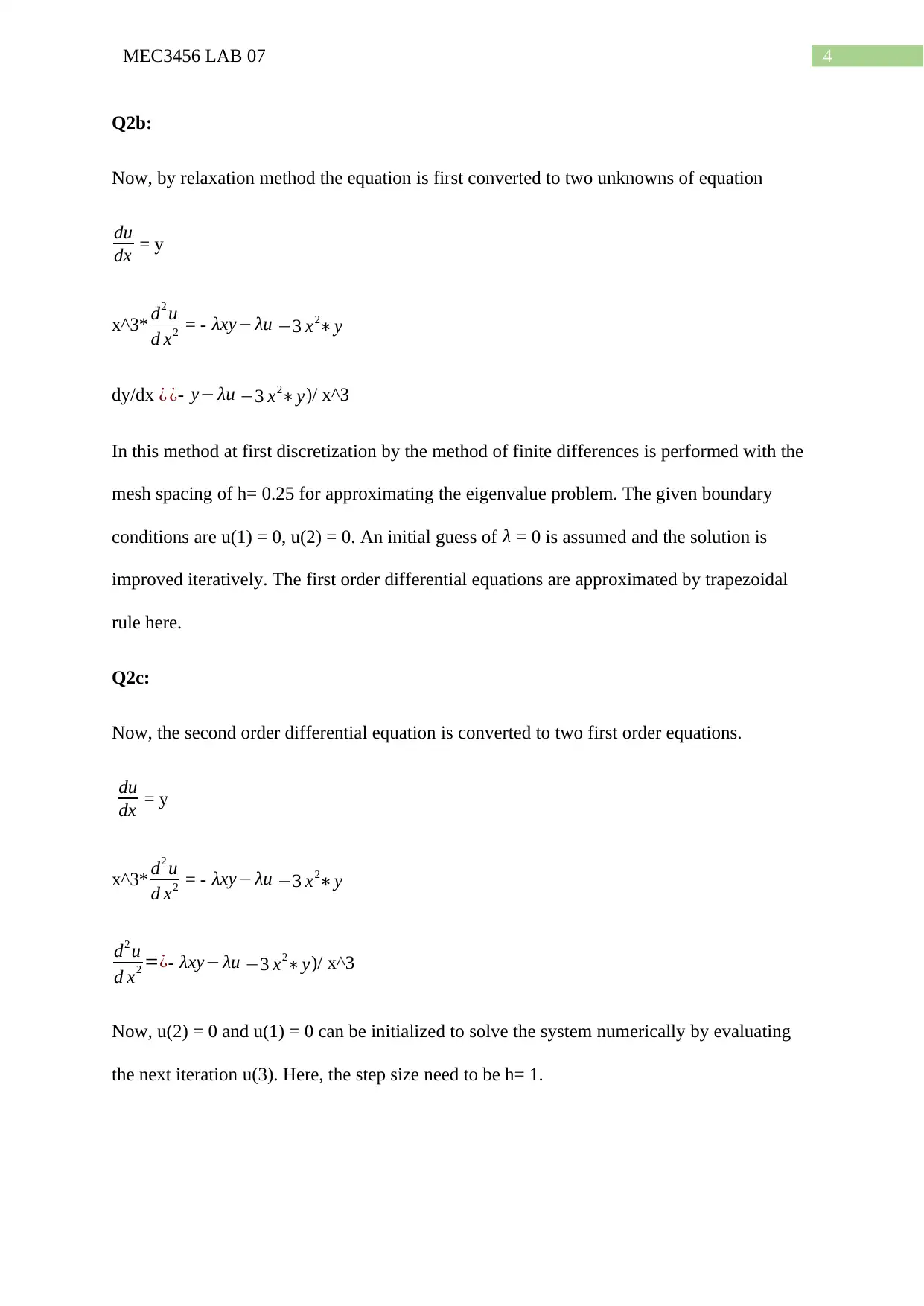
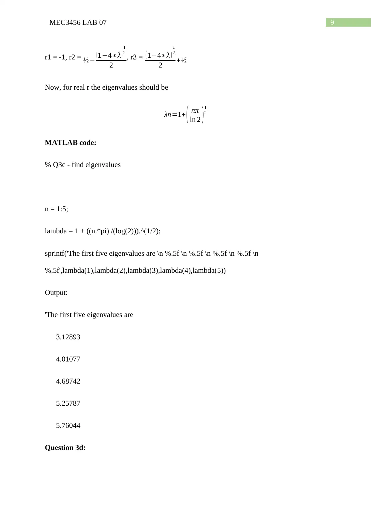
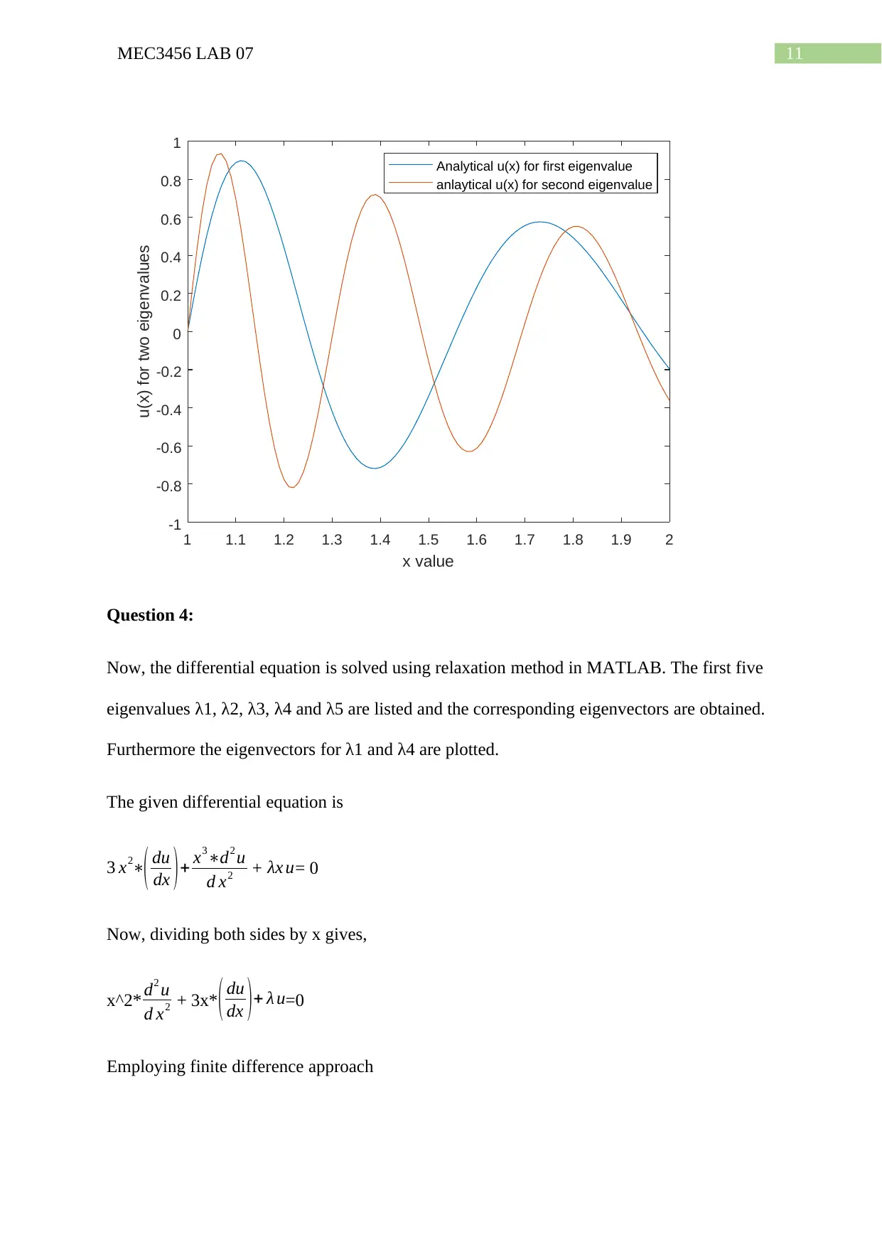
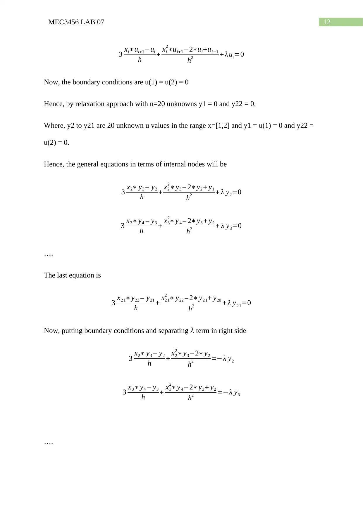
This assignment solution for MEC3456 Lab 07 focuses on solving ordinary differential equations (ODEs) using various numerical methods. The solution begins with the Adams-Bashforth method for solving an ODE, deriving the iteration equation using polynomial interpolation. It then addresses a second-order differential equation, applying the finite difference method and relaxation method for approximation. MATLAB code is provided to calculate the uRHS value and plot u(2) for a given eigenvalue range. The analytical solution for the Euler differential equation is derived, and the first five eigenvalues are calculated. The analytical solutions for the first and fourth eigenvalues are plotted. Finally, the assignment uses the relaxation method and MATLAB to solve the differential equation, listing the first five eigenvalues and plotting the corresponding eigenvectors for the first and fourth eigenvalues with different n values, demonstrating the impact of discretization on the solution.

Running head: MEC3456 LAB 07
MEC3456 LAB 07
Name of the Student
Name of the University
Author Note

2MEC3456 LAB 07
Question 1:
The Adams-Bashforth integration for finding the solution of the ODE dy/dt = f(t,y) are given
by the following integral update formula
yn+ 1= yn +∫
ti
ti+1
f ( t , y ) dt (1)
Where, yn+ 1 = y(tn+1 ¿
The method can be derived using polynomial interpretation as given below.
From equation (1) using the fundamental theorem of calculus we get
y(tn+1 ¿ = y(tn ¿ + ∫
tn
tn+1
y' ( t ) dt
Here, let A = ∫
tn
t n+1
y' ( t ) dt=∫
tn
t n+ 1
f (t , y ( t ) )dt
Now, for calculating the value of A the value of the interpolating polynomial P(t) as an
approximation f(t,y(t)) is used. Hence, the value of the interpolating polynomial in the
Lagrange form is
L(x) := ∑
j=0
k
yjlj(x ), where the expression of lj ( x )= ∏0 ≤m ≤ k∧m ≠ j
x −xm
xj−xm
Hence, the interpolation formula will be
P(t) = f ( tn , yn )∗t−tn−1
tn−tn−1
+f ( tn−1 , yn−1 )∗t−c
tn−1−tn
Hence, A = ∫
tn
tn+1
f ( t , y ( t ) ) dt ∫
tn
tn+1 f ( tn , yn ) ( t−tn−1 )
tn −tn−1
+ f ( tn−1 , yn−1 )∗t−tn
tn−1−tn
dt
Now, after integration and simplification gives,

3MEC3456 LAB 07
(½)(tn+tn +1 ¿ ( f ( tn , yn ) −f ( tn−1 , yn−1 ) )−tn−1 f ( tn , yn ) +tn f (tn−1 , yn−1)
= (½)( tn+ tn +1−2 tn−1 ¿ f ( tn , yn) + (½)(2tn−tn+1−t n ¿ f (tn−1 , yn−1 )
Now, tn−1 , c and tn+1 are equally spaced hence it can be considered that
tn−¿ tn−1 = tn+1−¿ tn = h. Hence, the value of A will be
A = (3/2)h*f( tn , yn ¿ – (½)h*f(tn−1 , yn−1 ¿
Hence, by Adams-Bashforth method the iteration equation will be this
y(tn+1 ¿ = y(tn ¿+ ( 3 h
2 )f ( tn , y n ) −( h
2 )f ( tn−1 , yn−1 )
Question 2:
2a:
The given second order differential equation is
( d
dx ) ( x3∗du
dx ) + λxu=0 (1)
The second order equation is defined inside the interval [1, 2] having boundary conditions
u(1) = 0 and u(2) = 0.
Hence, the above equation can be rewritten as
3 x2∗( du
dx )+ x3∗d2 u
d x2 + λx u= 0 (2)
Now, approximating (2) by finite difference method at an arbitrary point xi
3 xi
2∗ui+1 – ui
h + xi
3∗ui+1 – 2∗ui+ui−1
h2 + λ xi ui =0
Where, ui = u(xi) and holds true for all i.

4MEC3456 LAB 07
Q2b:
Now, by relaxation method the equation is first converted to two unknowns of equation
du
dx = y
x^3* d2 u
d x2 = - λxy− λu −3 x2∗y
dy/dx ¿ ¿- y− λu −3 x2∗y)/ x^3
In this method at first discretization by the method of finite differences is performed with the
mesh spacing of h= 0.25 for approximating the eigenvalue problem. The given boundary
conditions are u(1) = 0, u(2) = 0. An initial guess of λ = 0 is assumed and the solution is
improved iteratively. The first order differential equations are approximated by trapezoidal
rule here.
Q2c:
Now, the second order differential equation is converted to two first order equations.
du
dx = y
x^3* d2 u
d x2 = - λxy− λu −3 x2∗y
d2 u
d x2 =¿- λxy− λu −3 x2∗y)/ x^3
Now, u(2) = 0 and u(1) = 0 can be initialized to solve the system numerically by evaluating
the next iteration u(3). Here, the step size need to be h= 1.

5MEC3456 LAB 07
Here, any boundary condition can be chosen of u(1) and u’(1) as if u(x) is a solution of the
differential equation, then Cu(x) (C is any constant) is also a solution of the differential
equation. Now, for convenience we have chosen u(1) = 0 and u’(1) = 1.
Question 3a:
The uRHS value for x=2 for the differential equation is calculated by the following
MATLAB code.
MATLAB code:
function uRHS = RHS_Value(lambda)
% Calculates the RHS value of u given a guess for the eigenvalue lambda.
xspan = [1;2];
intcon = [0;1];
[x,u] = ode45(@odefunc,xspan,intcon);
uval = u(:,1);
% plot(x,uval,x,u(:,2))
% xlabel('x range in [1 2]')
% ylabel('solution u(x) and derivative du/dx')
% legend('u(x)','du/dx','Location','best')
uRHS = uval(end);

6MEC3456 LAB 07
function rhs = odefunc(x,u)
rhs = [u(2);(-lambda.*x.*u(2) - lambda.*u(1) - 3.*x.^2.*u(2))./(x.^3)];
end
end
Output:
uRHS =
0.2869
1 1.1 1.2 1.3 1.4 1.5 1.6 1.7 1.8 1.9 2
x range in [1 2]
0
0.1
0.2
0.3
0.4
0.5
0.6
0.7
0.8
0.9
1
solution u(x) and derivative du/dx
u(x)
du/dx
Question 3b:

7MEC3456 LAB 07
Now, for λ = [0,1000] the values of u(2) are plotted by the following code.
MATLAB code:
lambdarange = 0:1:1000;
for i=1:length(lambdarange)
uRHS(i) = RHS_Value(lambdarange(i));
end
figure(1)
plot(lambdarange,uRHS)
xlabel('\lambda')
ylabel('u(2)')
title('u value at x=2 for \lambda in [0,1000]')
Plot:

8MEC3456 LAB 07
0 100 200 300 400 500 600 700 800 900 1000
0
0.05
0.1
0.15
0.2
0.25
0.3
0.35
0.4
u(2)
u value at x=2 for in [0,1000]
Question 3c:
Given, differential equation
x^3* d2 u
d x2 = - λx∗du
dx − λu −3 x2∗du
dx
The above equation is of the form of Euler differential equation and the roots of the equation
that is required to be solved is
r(r-1)(r-2) + (3r*(r-1) + λr) + λ = 0
The solution has the form
u ( x ) =( 1
x )∗sin ( nπ∗ln ( x )
ln ( 2 ) )
Hence, solving for r gives,

9MEC3456 LAB 07
r1 = -1, r2 = ½− ( 1−4∗λ )
1
2
2
, r3 = ( 1 – 4∗λ )
1
2
2 +½
Now, for real r the eigenvalues should be
λn=1+ ( nπ
ln 2 ) 1
2
MATLAB code:
% Q3c - find eigenvalues
n = 1:5;
lambda = 1 + ((n.*pi)./(log(2))).^(1/2);
sprintf('The first five eigenvalues are \n %.5f \n %.5f \n %.5f \n %.5f \n
%.5f',lambda(1),lambda(2),lambda(3),lambda(4),lambda(5))
Output:
'The first five eigenvalues are
3.12893
4.01077
4.68742
5.25787
5.76044'
Question 3d:

10MEC3456 LAB 07
Now, for first and fourth eigenvalues the analytical solution is plotted by the following
MATLAB code.
MATLAB code:
lamdafirst = lambda(1); lamdafourth = lambda(4);
x = 1:0.01:2;
uvalfirst = x.^(-1).*sin(lamdafirst*pi*log(x)./log(2));
uvalfourth = x.^(-1).*sin(lamdafourth*pi*log(x)./log(2));
plot(x,uvalfirst)
hold on
plot(x,uvalfourth)
ylim([-1 1])
xlabel('x value')
ylabel('u(x) for two eigenvalues')
legend('Analytical u(x) for first eigenvalue','anlaytical u(x) for second eigenvalue')
Plot:

11MEC3456 LAB 07
1 1.1 1.2 1.3 1.4 1.5 1.6 1.7 1.8 1.9 2
x value
-1
-0.8
-0.6
-0.4
-0.2
0
0.2
0.4
0.6
0.8
1
u(x) for two eigenvalues
Analytical u(x) for first eigenvalue
anlaytical u(x) for second eigenvalue
Question 4:
Now, the differential equation is solved using relaxation method in MATLAB. The first five
eigenvalues λ1, λ2, λ3, λ4 and λ5 are listed and the corresponding eigenvectors are obtained.
Furthermore the eigenvectors for λ1 and λ4 are plotted.
The given differential equation is
3 x2∗( du
dx )+ x3∗d2 u
d x2 + λx u= 0
Now, dividing both sides by x gives,
x^2* d2 u
d x2 + 3x*( du
dx )+ λ u=0
Employing finite difference approach

12MEC3456 LAB 07
3 xi∗ui+1 – ui
h + xi
2∗ui+1 – 2∗ui+ui−1
h2 + λ ui=0
Now, the boundary conditions are u(1) = u(2) = 0
Hence, by relaxation approach with n=20 unknowns y1 = 0 and y22 = 0.
Where, y2 to y21 are 20 unknown u values in the range x=[1,2] and y1 = u(1) = 0 and y22 =
u(2) = 0.
Hence, the general equations in terms of internal nodes will be
3 x2∗ y3 – y2
h + x2
2∗y3 – 2∗y2 + y1
h2 + λ y2=0
3 x3∗y4 – y3
h + x3
2∗y 4 – 2∗y3 + y2
h2 + λ y3=0
….
The last equation is
3 x2 1∗y22 – y21
h + x2 1
2 ∗ y22 – 2∗y2 1+ y20
h2 + λ y2 1=0
Now, putting boundary conditions and separating λ term in right side
3 x2∗ y3 – y2
h + x2
2∗y3 – 2∗y2
h2 =−λ y2
3 x3∗y4 – y3
h + x3
2∗y 4 – 2∗y3 + y2
h2 =−λ y3
….