University Report: MECH2430 Residual Stress Measurement Analysis

This report presents an analysis of experimental data obtained from residual stress measurements using neutron diffraction. The study focuses on plastically deformed aluminum bars, specifically 6061-T6 and 7075-T6 alloys, subjected to 4-point bending. The report details the experimental setup, including sample preparation and deformation procedures. It includes material characterization from dog bone samples, stress calculations using Hooke's Law, and error analysis. The analysis involves processing tensile test data to establish elastic properties and characterize plastic behavior. The results are compared with expected distributions based on elastoplastic beam theory. The report also discusses the diffraction phenomenon, strain measurement techniques, and the application of neutron diffraction in measuring residual stress. The study utilizes MATLAB for data analysis and plotting, providing a comprehensive overview of the experimental process and findings.

Mechanical Engg.
MECH2430
Student Name –
Student ID –
Contents

Abstract/Executive Summary................................................................................................................2
Introduction and Background................................................................................................................3
Experiment Details................................................................................................................................6
Results and Data Analysis......................................................................................................................7
Material Characterisation from dog bone samples...........................................................................7
Stress calculation via Hooke’s Law...................................................................................................11
Error Analysis...................................................................................................................................14
Error analysis.......................................................................................................................................14
Residual Stress Calculation..............................................................................................................15
Discussion and Comparison.................................................................................................................16
Conclusions..........................................................................................................................................17
References...........................................................................................................................................17

Abstract/Executive Summary
In this project, the data obtained through the experiments is analysed and discussed. The data
obtained from the experiments which measure the residual stress for a beam that is deformed
plastically. The technique used is neutron diffraction. Firstly, the strain measuring methods
are discussed which are based on diffraction. Next, the data obtained from the experiments is
analysed and discussed based on elasto plastic beam bending. The analysis the experiments’
data provided is done for the calculation of the distribution of residual stress in each bar. The
tensile test data is processed for establishing the elastic properties and characterising the
plastic behaviour.
The Poisson's ratio is taken as 0.34 since it cannot be determined from the tensile test data.
On the calculation of the residual stress distribution in each bar, the results are compared to
the expected distributions based on elastoplastic beam theory.
Introduction and Background
Diffraction –
Diffraction occurs when there is an interaction between the waves and some geometrical
structures. There is a formation of alternate pattern due to constructive and destructive
interference which occurs between the waves which are created between the waves which are
created by 2 different sources. The quantum physics states that the subatomic particles like
photons, electrons, neutrons and protons show both particle as well as wave – like behaviour.

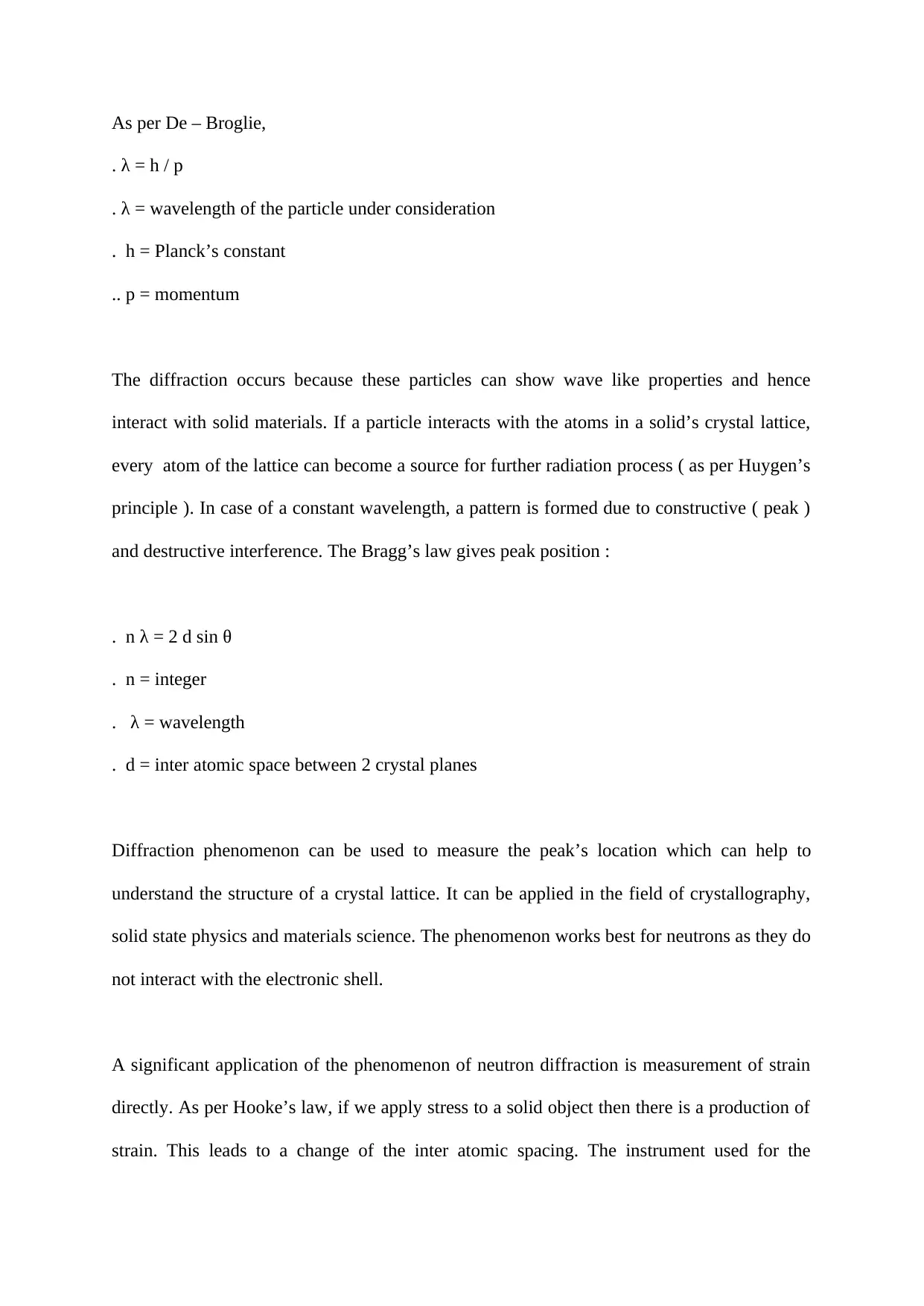
As per De – Broglie,
. λ = h / p
. λ = wavelength of the particle under consideration
. h = Planck’s constant
.. p = momentum
The diffraction occurs because these particles can show wave like properties and hence
interact with solid materials. If a particle interacts with the atoms in a solid’s crystal lattice,
every atom of the lattice can become a source for further radiation process ( as per Huygen’s
principle ). In case of a constant wavelength, a pattern is formed due to constructive ( peak )
and destructive interference. The Bragg’s law gives peak position :
. n λ = 2 d sin θ
. n = integer
. λ = wavelength
. d = inter atomic space between 2 crystal planes
Diffraction phenomenon can be used to measure the peak’s location which can help to
understand the structure of a crystal lattice. It can be applied in the field of crystallography,
solid state physics and materials science. The phenomenon works best for neutrons as they do
not interact with the electronic shell.
A significant application of the phenomenon of neutron diffraction is measurement of strain
directly. As per Hooke’s law, if we apply stress to a solid object then there is a production of
strain. This leads to a change of the inter atomic spacing. The instrument used for the

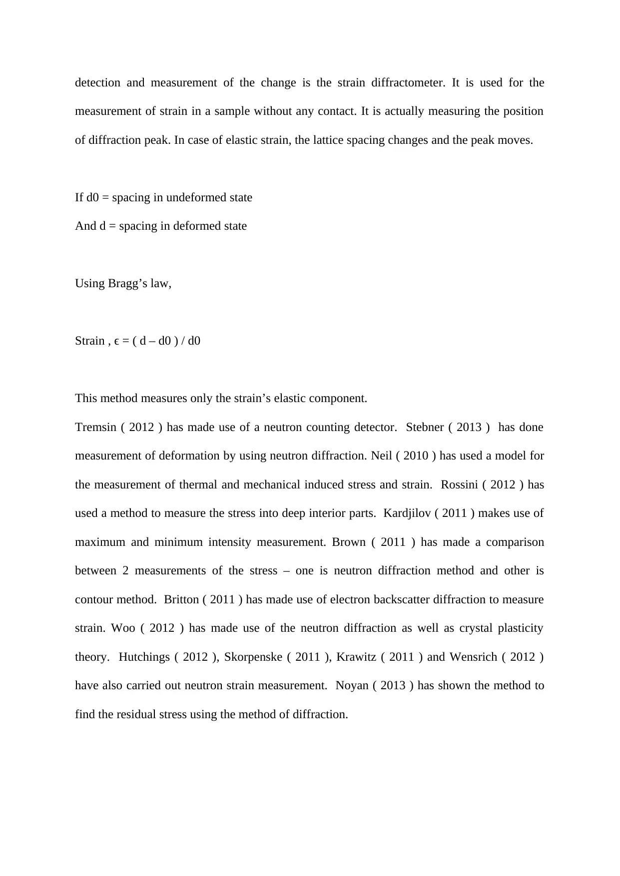
detection and measurement of the change is the strain diffractometer. It is used for the
measurement of strain in a sample without any contact. It is actually measuring the position
of diffraction peak. In case of elastic strain, the lattice spacing changes and the peak moves.
If d0 = spacing in undeformed state
And d = spacing in deformed state
Using Bragg’s law,
Strain , ϵ = ( d – d0 ) / d0
This method measures only the strain’s elastic component.
Tremsin ( 2012 ) has made use of a neutron counting detector. Stebner ( 2013 ) has done
measurement of deformation by using neutron diffraction. Neil ( 2010 ) has used a model for
the measurement of thermal and mechanical induced stress and strain. Rossini ( 2012 ) has
used a method to measure the stress into deep interior parts. Kardjilov ( 2011 ) makes use of
maximum and minimum intensity measurement. Brown ( 2011 ) has made a comparison
between 2 measurements of the stress – one is neutron diffraction method and other is
contour method. Britton ( 2011 ) has made use of electron backscatter diffraction to measure
strain. Woo ( 2012 ) has made use of the neutron diffraction as well as crystal plasticity
theory. Hutchings ( 2012 ), Skorpenske ( 2011 ), Krawitz ( 2011 ) and Wensrich ( 2012 )
have also carried out neutron strain measurement. Noyan ( 2013 ) has shown the method to
find the residual stress using the method of diffraction.

Experiment Details
Setup :
The experiment is based on neutron diffraction. The residual stress is measured in plastically
deformed aluminium bars using a KOWARI diffractometer in OPAL nuclear reactor Beam
Hall, Lucas Heights, Sydney, Australia.
Sample :
There are 2 samples of precipitation hardened aluminium alloys in the form of rectangular
bars. One sample is 6061 – T6 ( dimension – 40 mm x 44.45 mm x 300 mm ) and other
sample is 7075 – T6 ( dimension – 40 mm x 38.1 mm x 300 mm ). The 2 samples are
prepared on a milling machine and then polished. Then, they are deformed in 4 – pt bending
apparatus.
Then, alignment is done and load is slowly applied to both the samples till a maximum value
is reached and then removed. Deflection can be measured by using a small steel ruler. For the
sample 6061 – T6, the maximum load is 131 kN, maximum deflection is 7.2 mm and residual
deflection is 4.5 mm. For the sample 7075 – T6, the maximum load is 179 kN, maximum
deflection is 7 mm and residual deflection is 2.1 mm.
After being bent, both the samples are cut in 3 pieces of 100 mm length each. The central part
( deformed one ) kept as the sample to carry out the neutron diffraction experiment.

Results and Data Analysis
Material Characterisation from dog bone samples
Dog bones ( small samples ) are prepared to study the properties of the material. For the
sample 6061 – T6, the final load at rupture is 18.1 kN and maximum elongation is 0.2. For
the sample 7075 – T6, the final load at rupture is 34.7 kN and maximum elongation is 0.18.
The data obtained from the mechanical testing of dog bone samples is stored in 2 text files –
stress_strain_6061.txt and stress_strain_7075.txt. The files consist of 2 columns – length
measured by clip gauge ( in mm ) and applied load ( in kN ).
Firstly, the file ‘ stress_strain_6061.txt ’ is imported to MATLAB and then 2 columns are
converted to vectored columns. These can be analysed in the form of an array and plotted on
a graph using plot command. The axis can be labelled using ‘ label ’ command and suitable
title can be provided to the graph using the ‘ title ’ command.
Matlab Code :
Plot ( ClipGaugeLengthmm , ForcekN ) ;
Xlabel ( ' Gauge Length ( mm ) ' ) ;
Ylabel ( ' Force ( kN ) ' ) ;
Title ( ' Sample 6061 - T6 ' ) ;

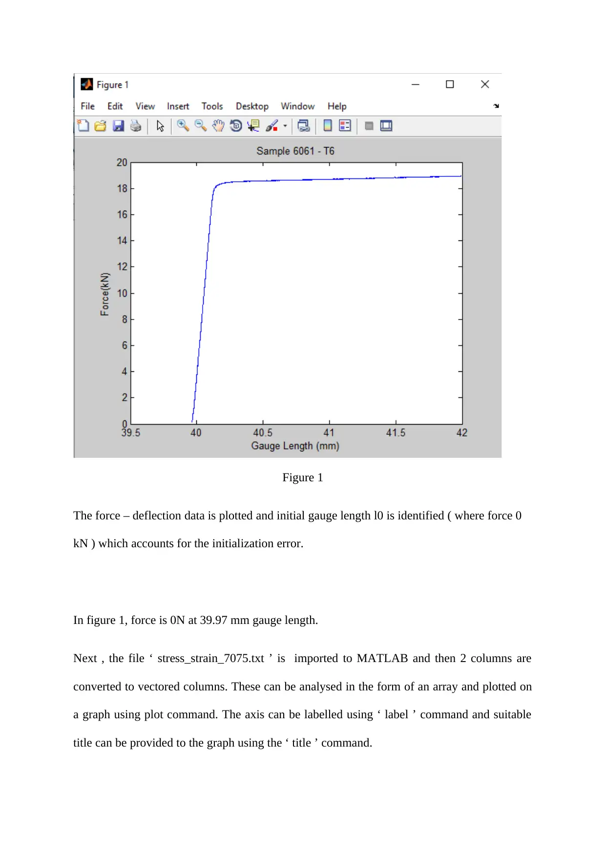
Figure 1
The force – deflection data is plotted and initial gauge length l0 is identified ( where force 0
kN ) which accounts for the initialization error.
In figure 1, force is 0N at 39.97 mm gauge length.
Next , the file ‘ stress_strain_7075.txt ’ is imported to MATLAB and then 2 columns are
converted to vectored columns. These can be analysed in the form of an array and plotted on
a graph using plot command. The axis can be labelled using ‘ label ’ command and suitable
title can be provided to the graph using the ‘ title ’ command.

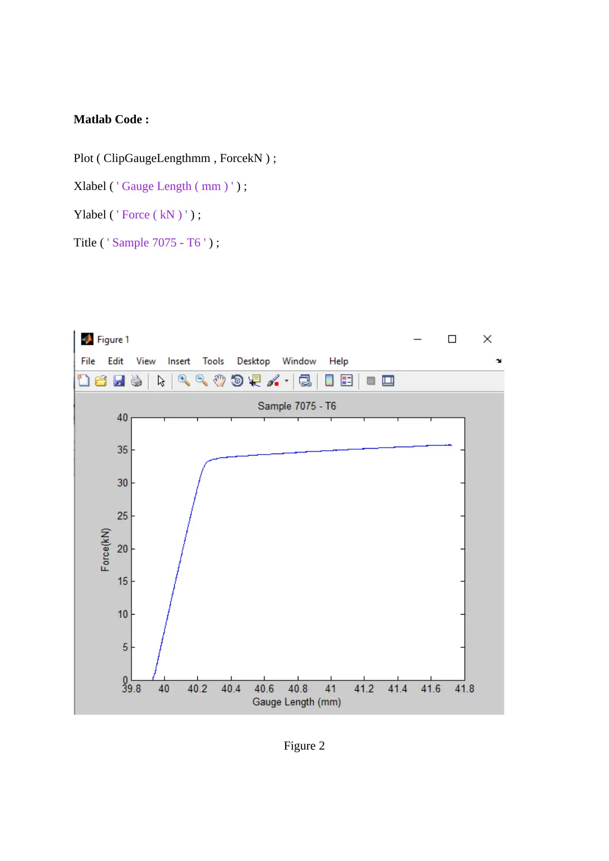
Matlab Code :
Plot ( ClipGaugeLengthmm , ForcekN ) ;
Xlabel ( ' Gauge Length ( mm ) ' ) ;
Ylabel ( ' Force ( kN ) ' ) ;
Title ( ' Sample 7075 - T6 ' ) ;
Figure 2

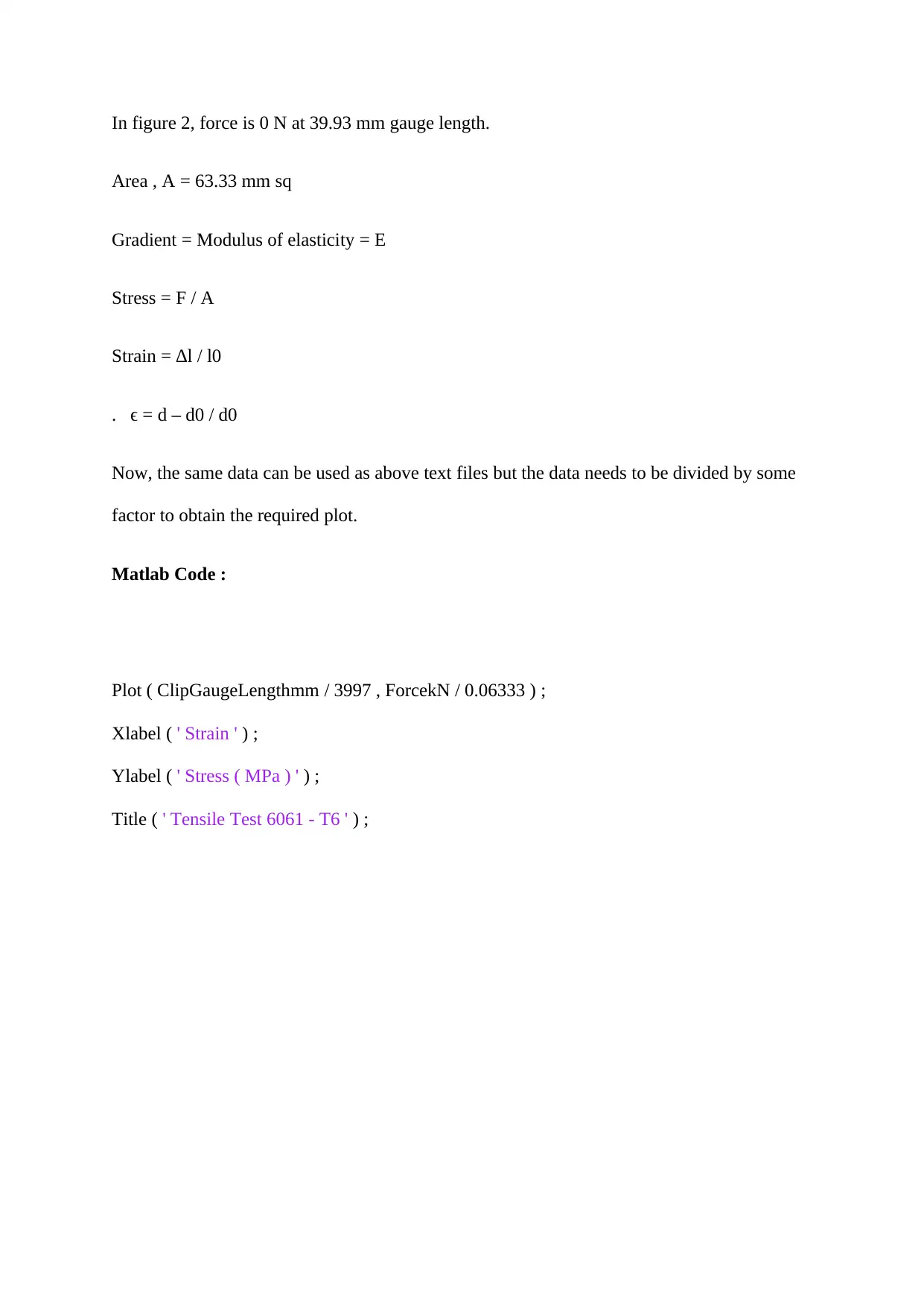
In figure 2, force is 0 N at 39.93 mm gauge length.
Area , A = 63.33 mm sq
Gradient = Modulus of elasticity = E
Stress = F / A
Strain = ∆l / l0
. ϵ = d – d0 / d0
Now, the same data can be used as above text files but the data needs to be divided by some
factor to obtain the required plot.
Matlab Code :
Plot ( ClipGaugeLengthmm / 3997 , ForcekN / 0.06333 ) ;
Xlabel ( ' Strain ' ) ;
Ylabel ( ' Stress ( MPa ) ' ) ;
Title ( ' Tensile Test 6061 - T6 ' ) ;

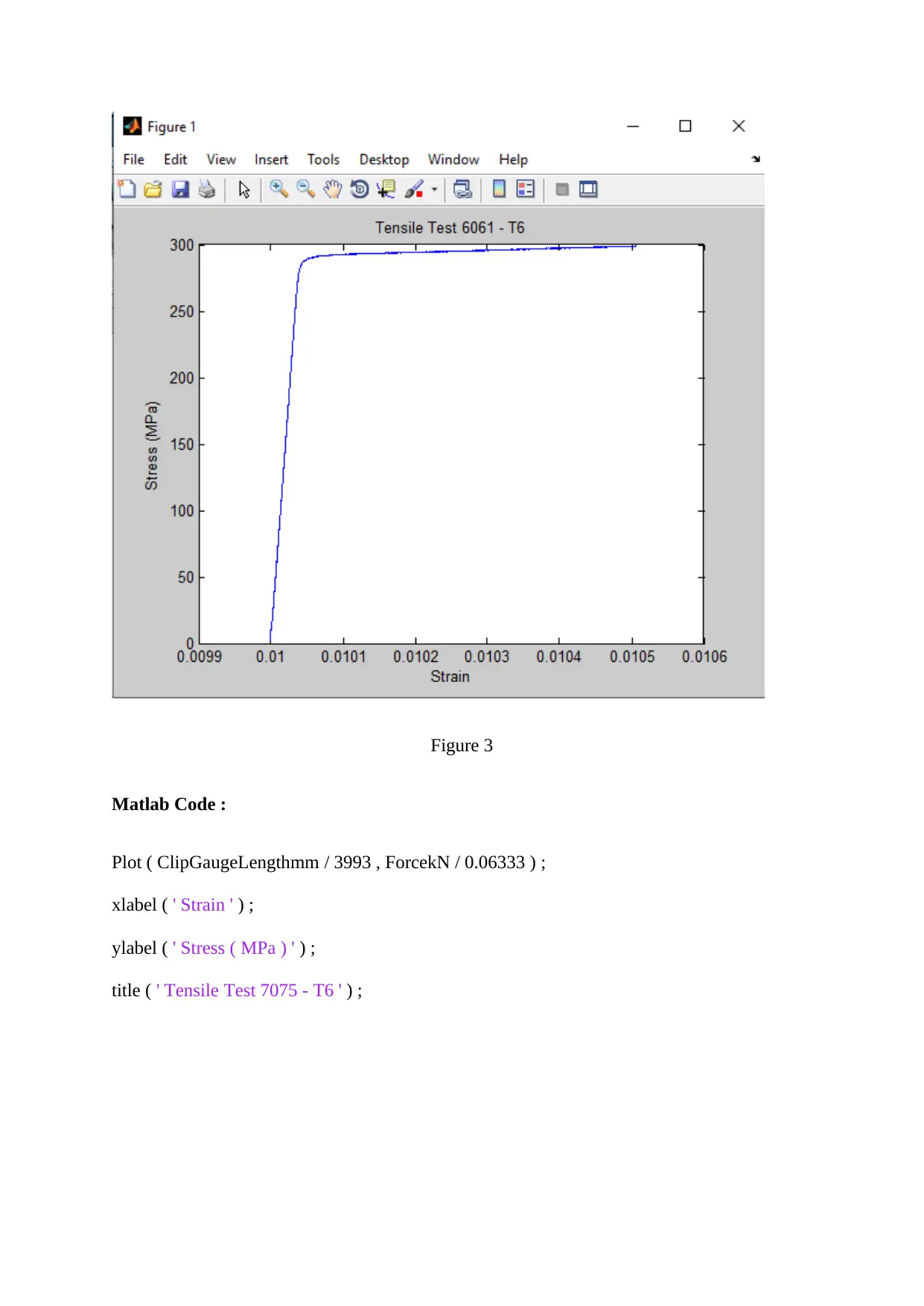
Figure 3
Matlab Code :
Plot ( ClipGaugeLengthmm / 3993 , ForcekN / 0.06333 ) ;
xlabel ( ' Strain ' ) ;
ylabel ( ' Stress ( MPa ) ' ) ;
title ( ' Tensile Test 7075 - T6 ' ) ;

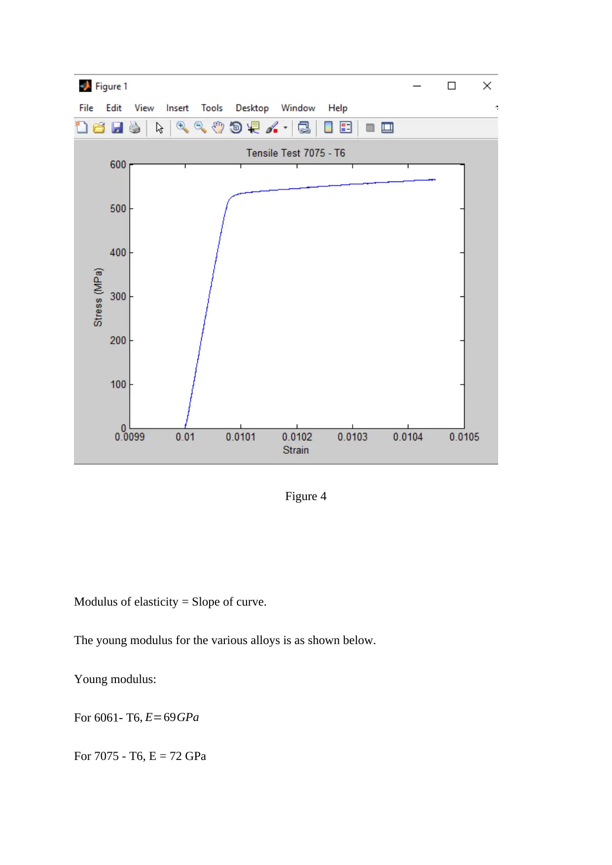
Figure 4
Modulus of elasticity = Slope of curve.
The young modulus for the various alloys is as shown below.
Young modulus:
For 6061- T6, E=69GPa
For 7075 - T6, E = 72 GPa