Mechanical Engineering: Heat Exchanger CFD Simulation Project

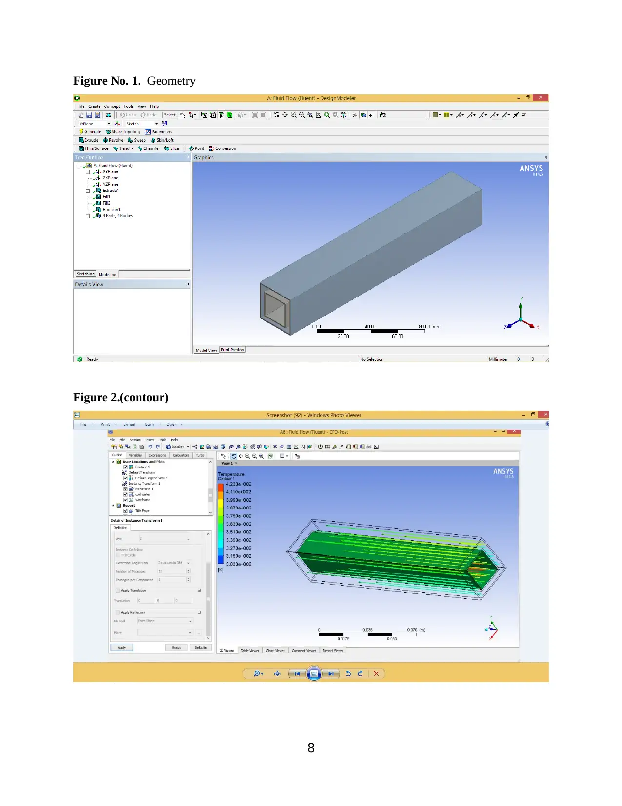
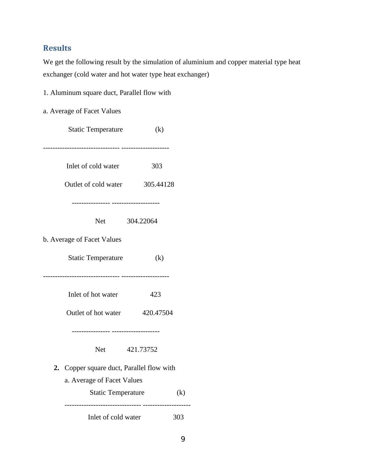
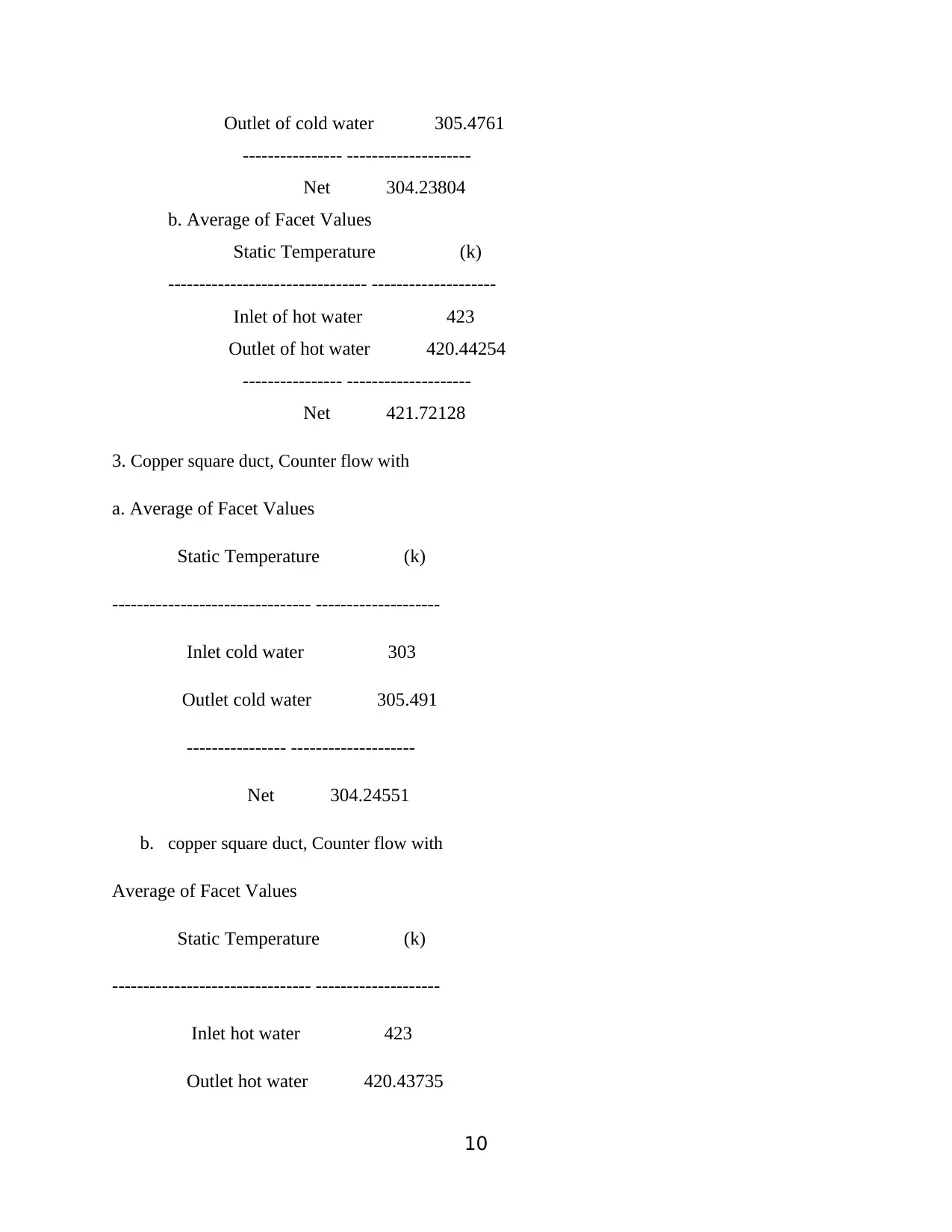
This project details a Computational Fluid Dynamics (CFD) analysis of a heat exchanger, outlining the objectives, methodology, and results. The primary goal is to simulate and analyze the temperature, pressure, and velocity of fluids within the heat exchanger, comparing aluminum and copper materials in both parallel and counter flow configurations. The methodology involves creating a 3D model in SolidWorks, importing it into ANSYS Workbench, and utilizing the Fluid Flow (Fluent) module. Key steps include meshing, setting up boundary conditions, defining material properties, and running the simulation. The results section presents the average facet values for static temperature at the inlet and outlet of both hot and cold water, for both materials and flow arrangements, and includes stream flow and contour graphs. The project highlights the advantages of CFD, such as cost and time savings, while acknowledging its disadvantages, like the need for skilled users and the cost of software.

General Information
1. The objective of the simulation:- Main objective of CFD analysis is following
a. Find the inlet and outlet temperature of hot pipe and cold pipe and their difference.
b. Find the inlet and outlet pressure of hot pipe and cold pipe fluid and their difference.
c. Find the inlet and outlet velocity of fluid in hot pipe and cold pipe and their difference.
d. Generate the graph of stream flow of fluid
e. Generate the graph of contour flow (Munson, 2007)
Methodology
We follow the following step to analyses the heat exchanger in CFD module of ansys in work
wench.
Step1. Generate 3d model in solid works software with given dimension.
Step 2. Start workbench of ansys software.
Step3. Used fluid flow (fluent)

Step 4: import the geometry or create the geometry then fill the martial like fluid inside
the pipe the re generate the geometry.
Step 5: shutdown the design modeller.
Step 6: start the mesh module
Setting the value of module
1. Defaults value like physics preference and relevance value.
1

2. Set the value following value of sizing
a. Use advance value of size function
b. Relevance centre
c. Initial size seed
d. Smoothing
e. Span angle centre
f. Curvature normal angle
g. Min size
h. Max size
i. Growth rate
j. Minimum edge length
3. Set the inflation value
a. Use automatic inflation
b. Inflation option
c. Transition ratio
d. Maximum layers
e. Growth rate
f. Inflation algorithm
g. View advance option
4. Patch conforming options
a. Triangle surface mesher
5. Advanced
a. shape checking
b. element mid side nodes
c. straight sided element
d. number of retries
e. extra retries for assembly
f. rigid body behaviour
g. mesh morphing
6. Disfeaturing
a. Pinch tolerance
2

b. Generate pinch of reference
c. Automatic mesh based defeaturing
d. Defeaturing tolerance
7. Statics
a. Nodes
b. Elements
c. Mesh metric
Step 8. Shutdown the close meshing
Step 9. Open the setup
Set the value of following feature
a. General
b. Models and take the following value of models
1. Multiphase
2. Energy
3. Viscous
4. Radiation
3

5. Heat exchanger
6. Specie
7. Discrete phase
8. Solidification and melting
9. Acoustics
10. Eulerian wall film
c. Material – assign the following material according to our requirement.
1. Fluid – water – liquid select
2. Solid- copper and aluminium
d. Cell zone condition – assign the material of pipe and water according to our requirement
and assignment temperature also
Like. Temperature of inlet hot water = 423 kelvin
Temperature of inlet cold water = 303 kelvin
Material of pipe – aluminium & copper chose according to our requirement.
e. Set the boundary condition
1. Inlet hot water
2. Outlet hot water
3. Inlet wall
4. Outlet wall
f. Mesh interface
g. Dynamic mesh
h. Reference value
Step. 10 solution
1. Solution method
Take the value
Scheme = simple
Spatial discretization
Gradient = least square cell based
Pressure = standard
Momentum = second order upwind
Turbulent kinetic energy = first order upwind
4

Turbulent dissipation rate = first order upwind
2. Solution controls
Pressure = 0.3
Density = 1
Body force = 1
Momentum = 0.7
Turbulent kinetic energy =0.8
3. Monitors
4. Solution initialization
a. Initialization method = standard initialization
b. Compute from = inlet
c. Reference frame = relative to cell zone
d. Gauge pressure (Pascal) = 0
e. X velocity = 0
f. y velocity = 0
g. z velocity = 0
h. turbulent kinetic energy = 0.02261741
i. turbulent dissipation rate = 4.58894
Then initialize
j. run calculation
Number of iteration = 28, reporting interval = 1 and profile updated interval = 1
the calculate (G., 2017)
5

Step 10: shutdown the setup
Step 11. Start the result window
a. select the stream line and set all value according to our requirement for hot water
1. type = 3d stream
2. domains = all domain
3. start from = inlet of hot water
4. sampling = equal spaced
5. # point = 25
6. Variable = velocity and temperature
b. select the stream line and set all value according to our requirement for hot water
7. type = 3d stream
8. domains = all domain
9. start from = inlet of cold water
10. sampling = equal spaced
11. # point = 25
6

12. Variable = velocity and temperature
c. Select the contour and select the all value according to our requirement
1. Domain = all domains
2. Location = contact region
3. Variable = temperature, pressure, velocity, density etc.
4. Range = global
7

Figure No. 1. Geometry
Figure 2.(contour)
8

Results
We get the following result by the simulation of aluminium and copper material type heat
exchanger (cold water and hot water type heat exchanger)
1. Aluminum square duct, Parallel flow with
a. Average of Facet Values
Static Temperature (k)
-------------------------------- --------------------
Inlet of cold water 303
Outlet of cold water 305.44128
---------------- --------------------
Net 304.22064
b. Average of Facet Values
Static Temperature (k)
-------------------------------- --------------------
Inlet of hot water 423
Outlet of hot water 420.47504
---------------- --------------------
Net 421.73752
2. Copper square duct, Parallel flow with
a. Average of Facet Values
Static Temperature (k)
-------------------------------- --------------------
Inlet of cold water 303
9

Outlet of cold water 305.4761
---------------- --------------------
Net 304.23804
b. Average of Facet Values
Static Temperature (k)
-------------------------------- --------------------
Inlet of hot water 423
Outlet of hot water 420.44254
---------------- --------------------
Net 421.72128
3. Copper square duct, Counter flow with
a. Average of Facet Values
Static Temperature (k)
-------------------------------- --------------------
Inlet cold water 303
Outlet cold water 305.491
---------------- --------------------
Net 304.24551
b. copper square duct, Counter flow with
Average of Facet Values
Static Temperature (k)
-------------------------------- --------------------
Inlet hot water 423
Outlet hot water 420.43735
10

---------------- --------------------
Net 421.71866
4 Aluminium square duct, Counter flow with
a. Hot water
Inlet hot water 423
Outlet hot water 420.47198
---------------- --------------------
Net 421.73599
b. cold water
Inlet cold water 303
Outlet cold water 305.45679
---------------- --------------------
Net 304.22839
Advantage of CFD:
1. It is saving the cost of new product development.
2. It is saving the time. (it is not hit and trial method)
3. It is provide approximately accurate result.
4. Material saving during new product development.
Disadvantage of CFD:
1. It is require skill person to handle the software.
2. Software is costly.
3. Small industry cannot handle that type of software. (S. Yoshimoto, 2011)
11

12