Analysis of Wood Burning Rate Experiment and Results

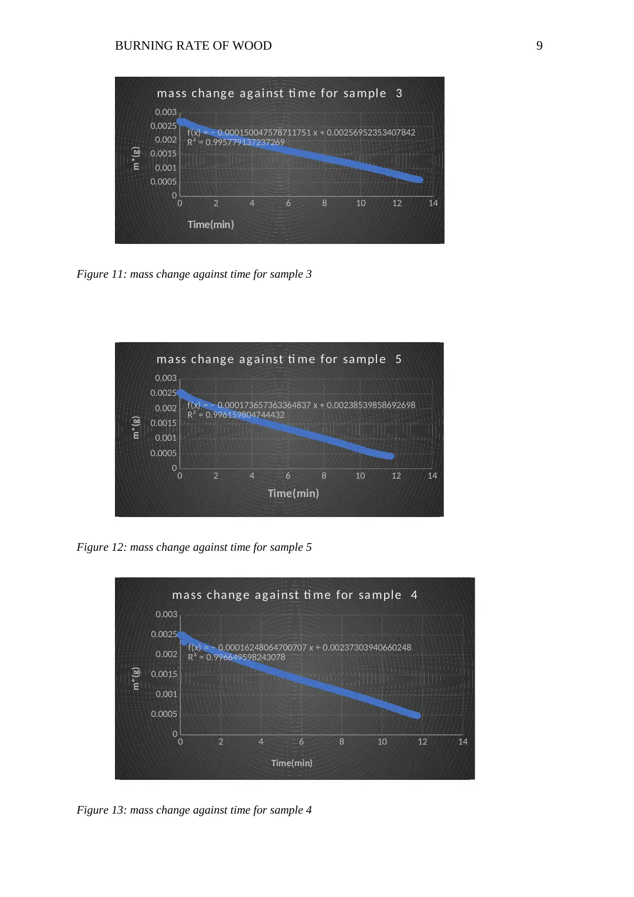
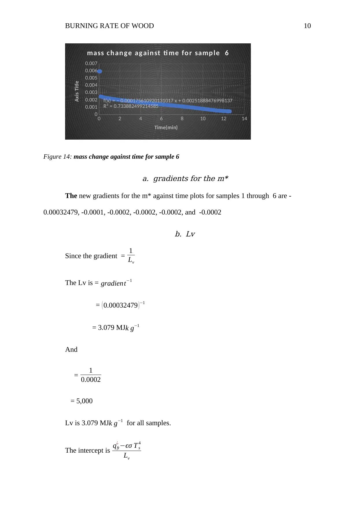
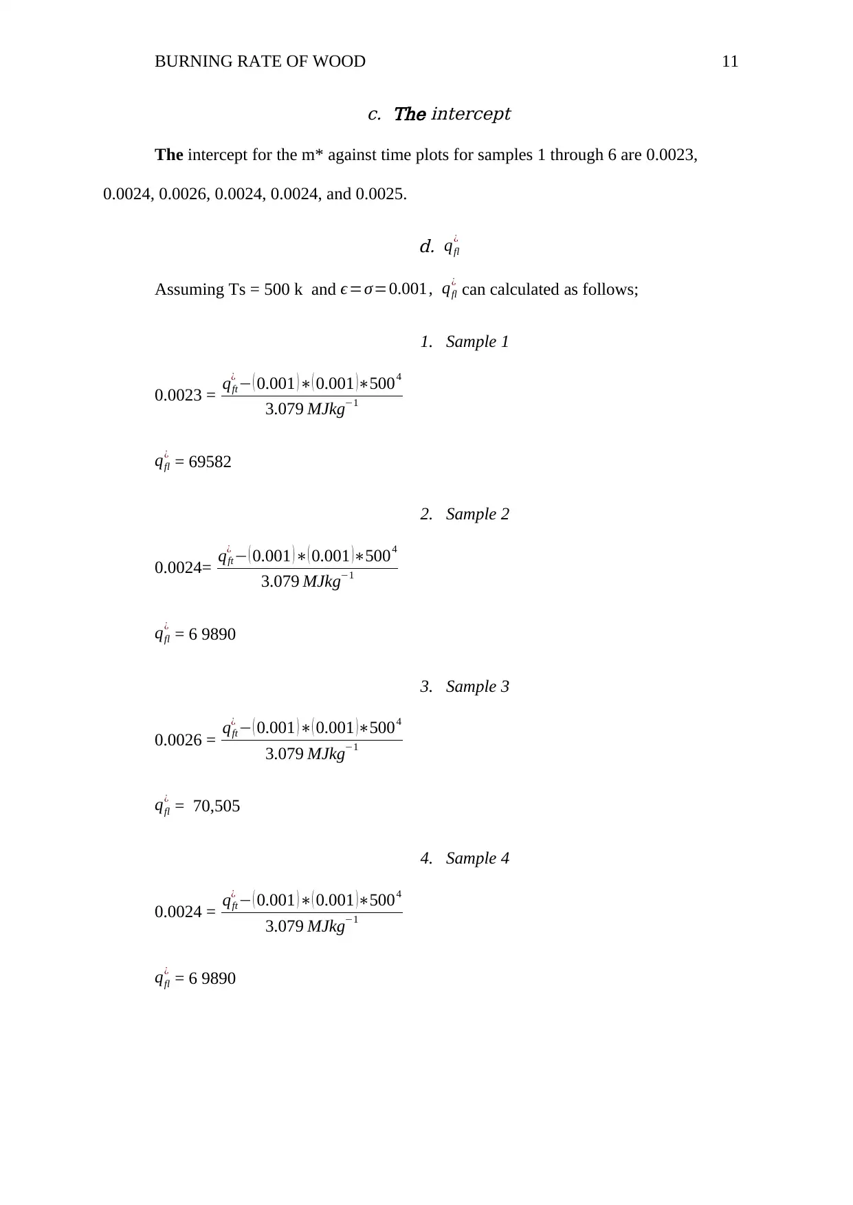
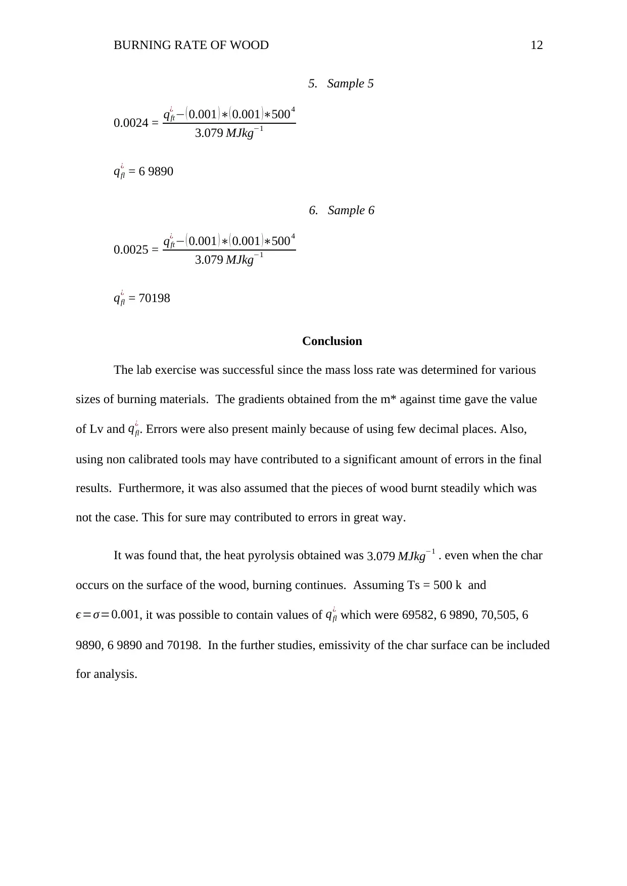
This assignment analyzes a practical experiment on the burning rate of wood, conducted to investigate mass loss under varying heat fluxes. The experiment used a cone heater and measured the mass loss of wood samples with different dimensions. The report details the methodology, including the apparatus, procedure, and data collection. Results are presented in tables and graphs, showing the relationship between mass change and time. The analysis includes the calculation of gradients, heat of gasification (Lv), and surface temperatures. The report discusses the findings, potential sources of error, and the limitations of the experiment, concluding with suggestions for further research such as including the emissivity of the char surface for analysis. The analysis is based on data from six samples at different temperatures and the provided data files.

Running Head: BURNING RATE OF WOOD
BURNING RATE OF WOOD
Name
Institute of Affiliation
Date

BURNING RATE OF WOOD 2
Introduction
Continuous burning takes place in solid materials if the thermal energy feedback to
surface of the materials emits volatiles which causes the burning to continues. Mean mass
reduction for the burning material is a function of the external flux, heat losses on the surface
and heat flux from the burning frame. Effective gasification of the material defines the
thermal energy that is needed to produce 1kg of the volatiles at give temperature T v over a
given period of time where energy balance approach is used. Equation 1 shows the
expression of the mass loss rate for the system (Peacock, Davis & Babrauskas, 2011).
The objective of this lab exercise is to investigate the mass loss of pieces of wood that
have different areas and dimensions. The results are then plotted to visualizes the effect.
Theory
One-dimension heating equation for the mass burning rate is given as shown below;
˙m¿= m
As
. . . . . . . . . . . . . . . . . . . . . . . . . . . . . . . . . . . . . . . . . . . . . . . . . . . . . . . . . . .Equation 1
Where ˙m¿ is the mass burning rate per unit area, and As surface are of the sample set
in the horizontal orientation… A mass loss graph for would have a general trend as shown in
the figure 1 below.
Figure 1: Typical mass loss for a given piece of wood.

BURNING RATE OF WOOD 3
The steady mass loss rate can be estimated by use of the formula shown below;
˙m¿= ˙qnet
Lv
. . . . . . . . . . . . .. . . . . .. . . . . . . . . . . . . . . . . . . . . . . . . . . . . . . . . . . . . . .Equation 2
Where ˙qnet is net heat flux to the surface of the burning material and Lv is the heat of
gasification. The above equation can be rewritten as shown below;
˙m¿= qe
¿+ qft
¿ −ϵσ T s
4
Lv
. . . . . . .. . . . . . . . . . . . . . . . . . . . . . . . . . . . . . . . . . . . . . . . . . . . . . . . . Equation
3
Where T s is the surface temperature and qfl
¿ is the heat flux of the flame … For a non-
charring material, the surface temperature would be fixed pyrosis temperature. If the heat
flux of the flame qfl
¿ and surface temperature T s are assumed to be constant, equation 3 can
be rearranged as follows;
˙m¿= qe
¿
Lv
+ qft
¿ −ϵσ T s
4
Lv
. . . . . . .. . . . . . . . . . . . . . . . . . . . . . . . . . . . . . . . . . . . . . . . . . . . . . .Equation 4
If equation 4 is plotted, 1
Lv
would be the slope and qft
¿ −ϵσ T s
4
Lv
would be the y
intercept.
Methodology
a. Apparatus
1. Cone heaters
2. Spark igniter
3. Load cell
4. Timer

BURNING RATE OF WOOD 4
b. Procedure
A new record file was generated on the computer. The cone heater temperature was
set to 650° C. the ˙qe was measured using the radiometer. The sample had their mass and
dimension measured and recorded on the table. The tray under the cone heater was first
crossed and the load cell set to zero. After the shutter was opened, ignition was started and
immediately recording was done on the computer. Using the computer, the mass history of
the wood is recorded. The experiment was repeated now after the temperatures were set to
850 ° at a step interval of 50 ° C.
Results
The mass and dimensions are as follows;
Table 1: The samples` dimension, mass and het flux
Sample Length Width
Thicknes
s
As(mm2
) As(m2)
1 74 73 18 16096
0.01609
6
2 75 73 18 16278
0.01627
8
3 75 74 18 16464
0.01646
4
4 74 74 17 15984
0.01598
4
5 74 72 18 15912
0.01591
2
6 77 76 18 17212
0.01721
2
Graphs as follows;

BURNING RATE OF WOOD 5
0 2 4 6 8 10 12 14 16 18 20
0
10
20
30
40
50
f(x) = − 1.78600968201115 x + 37.3418597111701
R² = 0.995114821607419
mass change against time for sample
1
Time (min)
change in mass
Figure 2: mass change against time for sample 1
0 2 4 6 8 10 12 14 16 18
0
5
10
15
20
25
30
35
40
45
f(x) = − 2.17099836763617 x + 39.5693434718101
R² = 0.987174542692138
mass change against time for sample 2
Time (min)
change in mass
Figure 3: mass change against time for sample 2

BURNING RATE OF WOOD 6
0 2 4 6 8 10 12 14
0
10
20
30
40
50
f(x) = − 2.47038333591027 x + 42.3046354650672
R² = 0.995779137237269
mass change against time for sample 3
Time (min)
change in mass
Figure 4: mass change against time for sample 3
0 2 4 6 8 10 12 14
0
10
20
30
40
f(x) = − 2.76323596586128 x + 37.9564623151821
R² = 0.996159804744432
mass change against time for sample 5
Time (min)
change in mass
Figure 5: mass change against time for sample 5

BURNING RATE OF WOOD 7
0 2 4 6 8 10 12 14
0
5
10
15
20
25
30
35
40
45
f(x) = − 2.59709066176101 x + 37.9306618751341
R² = 0.996649598243078
mass change against time for sample 4
Time (min)
change in mass
Figure 6: mass change against time for sample 4
0 2 4 6 8 10 12 14
0
20
40
60
80
100
120
f(x) = − 3.02261515729506 x + 43.3550446609193
R² = 0.733882499214585
mass change against time for sample 6
Time (min)
change in mass
Figure 7: mass change against time for sample 6
The gradients for the mass against time plots for samples 1 through 6 are -1.786,-
2.171, -2.4704 , - 2.597 , -2.7632, and -3.022 respectively. Below is a comparison graph for
all the sample

BURNING RATE OF WOOD 8
Figure 8: Comparison graph for all samples ( plotted using MATLAB)
Below is m* against time
0 2 4 6 8 10 12 14 16 18 20
0
0.0005
0.001
0.0015
0.002
0.0025
0.003
f(x) = − 0.0001109598460494 x + 0.00231994655263233
R² = 0.995114821607419
ma ss cha ng e a g ai nst ti me for sa mpl e 1
Time(min)
m*(g)
Figure 9: mass change against time for sample 1
0 2 4 6 8 10 12 14 16 18
0
0.0005
0.001
0.0015
0.002
0.0025
0.003
f(x) = − 0.000133370092618023 x + 0.00243084798327866
R² = 0.987174542692138
ma ss cha ng e ag a i nst ti me for sa mpl e 2
Time(min)
m(g)
Figure 10: mass change against time for sample 2

BURNING RATE OF WOOD 9
0 2 4 6 8 10 12 14
0
0.0005
0.001
0.0015
0.002
0.0025
0.003
f(x) = − 0.000150047578711751 x + 0.00256952353407842
R² = 0.995779137237269
ma ss cha ng e a g ai nst ti me for sa mpl e 3
Time(min)
m*(g)
Figure 11: mass change against time for sample 3
0 2 4 6 8 10 12 14
0
0.0005
0.001
0.0015
0.002
0.0025
0.003
f(x) = − 0.000173657363364837 x + 0.00238539858692698
R² = 0.996159804744432
ma ss cha ng e a g ai nst ti me for sa mpl e 5
Time(min)
m*(g)
Figure 12: mass change against time for sample 5
0 2 4 6 8 10 12 14
0
0.0005
0.001
0.0015
0.002
0.0025
0.003
f(x) = − 0.00016248064700707 x + 0.00237303940660248
R² = 0.996649598243078
ma ss cha ng e a g ai nst ti me for sa mple 4
Time(min)
m*(g)
Figure 13: mass change against time for sample 4

BURNING RATE OF WOOD 10
0 2 4 6 8 10 12 14
0
0.001
0.002
0.003
0.004
0.005
0.006
0.007
f(x) = − 0.000175610920131017 x + 0.00251888476998137
R² = 0.733882499214585
mass ch an g e ag ain st ti me fo r samp le 6
Time(min)
Axis Title
Figure 14: mass change against time for sample 6
a. gradients for the m*
The new gradients for the m* against time plots for samples 1 through 6 are -
0.00032479, -0.0001, -0.0002, -0.0002, -0.0002, and -0.0002
b. Lv
Since the gradient = 1
Lv
The Lv is = gradient−1
= ( 0.00032479 ) −1
= 3.079 MJk g−1
And
= 1
0.0002
= 5,000
Lv is 3.079 MJk g−1 for all samples.
The intercept is qft
¿ −ϵσ T s
4
Lv

BURNING RATE OF WOOD 11
c. The intercept
The intercept for the m* against time plots for samples 1 through 6 are 0.0023,
0.0024, 0.0026, 0.0024, 0.0024, and 0.0025.
d. qfl
¿
Assuming Ts = 500 k and ϵ=σ=0.001, qfl
¿ can calculated as follows;
1. Sample 1
0.0023 = qft
¿ − ( 0.001 )∗( 0.001 )∗5004
3.079 MJkg−1
qfl
¿ = 69582
2. Sample 2
0.0024= qft
¿ − ( 0.001 )∗( 0.001 )∗5004
3.079 MJkg−1
qfl
¿ = 6 9890
3. Sample 3
0.0026 = qft
¿ − ( 0.001 )∗( 0.001 )∗5004
3.079 MJkg−1
qfl
¿ = 70,505
4. Sample 4
0.0024 = qft
¿ − ( 0.001 )∗( 0.001 )∗5004
3.079 MJkg−1
qfl
¿ = 6 9890

BURNING RATE OF WOOD 12
5. Sample 5
0.0024 = qft
¿ − ( 0.001 )∗( 0.001 )∗5004
3.079 MJkg−1
qfl
¿ = 6 9890
6. Sample 6
0.0025 = qft
¿ − ( 0.001 )∗( 0.001 )∗5004
3.079 MJkg−1
qfl
¿ = 70198
Conclusion
The lab exercise was successful since the mass loss rate was determined for various
sizes of burning materials. The gradients obtained from the m* against time gave the value
of Lv and qfl
¿ . Errors were also present mainly because of using few decimal places. Also,
using non calibrated tools may have contributed to a significant amount of errors in the final
results. Furthermore, it was also assumed that the pieces of wood burnt steadily which was
not the case. This for sure may contributed to errors in great way.
It was found that, the heat pyrolysis obtained was 3.079 MJkg−1 . even when the char
occurs on the surface of the wood, burning continues. Assuming Ts = 500 k and
ϵ=σ=0.001, it was possible to contain values of qfl
¿ which were 69582, 6 9890, 70,505, 6
9890, 6 9890 and 70198. In the further studies, emissivity of the char surface can be included
for analysis.