Analysis of a Motorbike 2 DOF Dynamic System in Mechanical Engineering

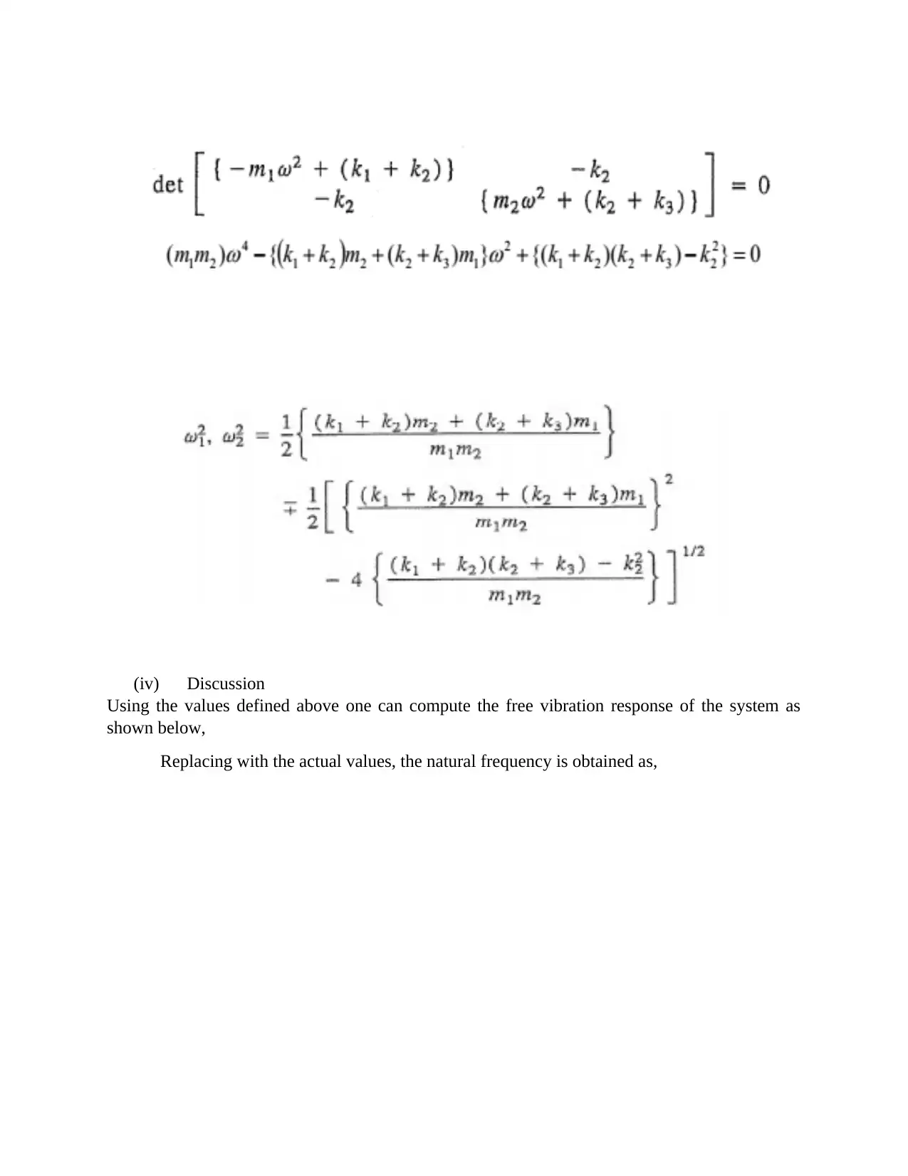
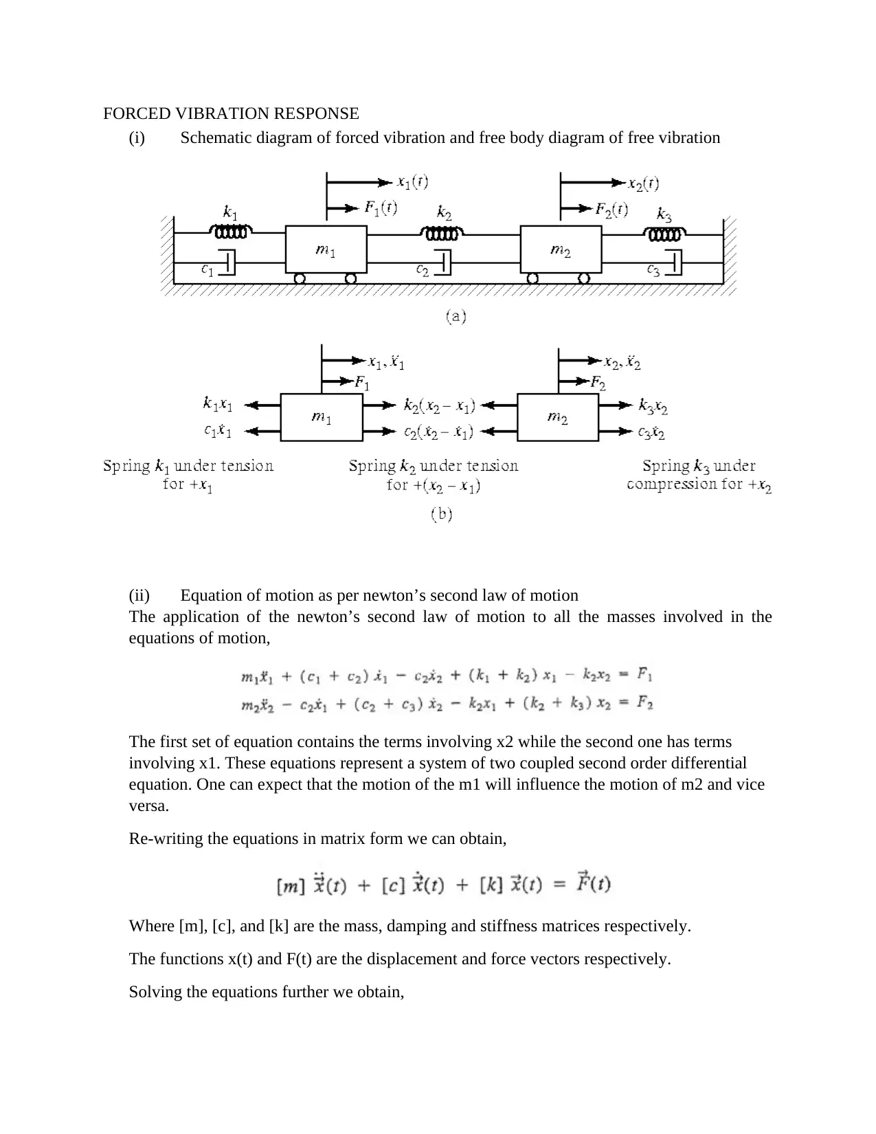
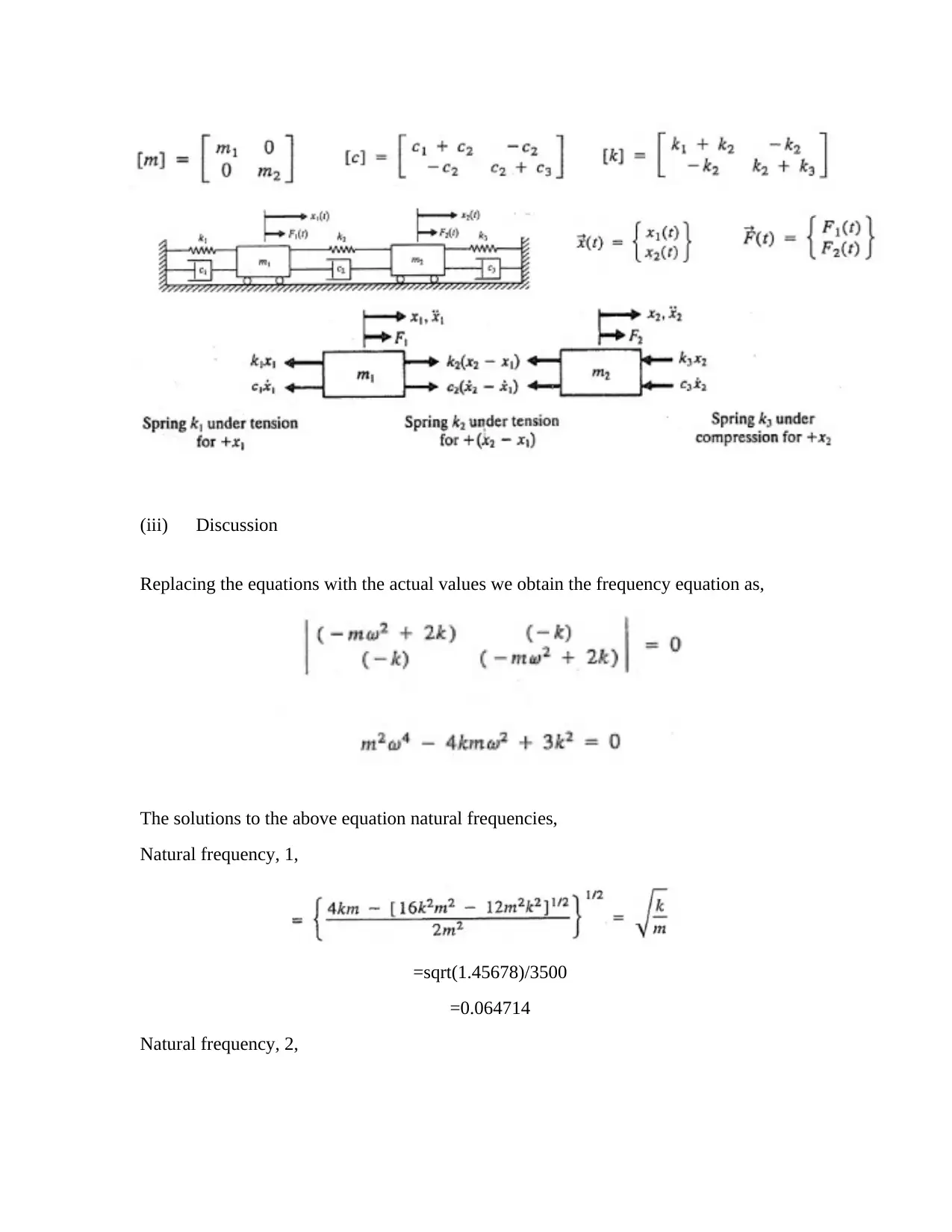
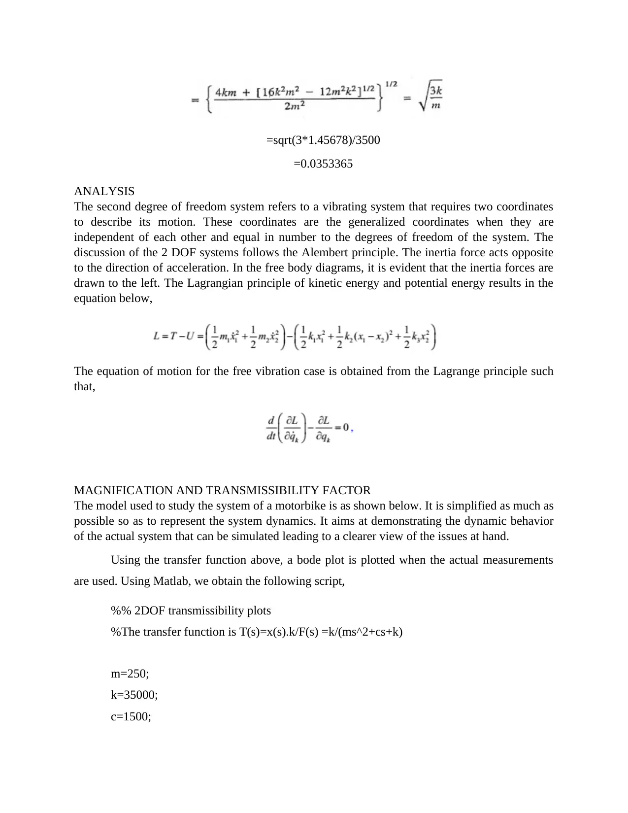
This project presents a detailed analysis of a motorbike's second-degree-of-freedom (2 DOF) dynamic system. The study utilizes MATLAB and Simulink to model and analyze the motorbike's behavior, focusing on free and forced vibration responses. The project includes schematic diagrams, free body diagrams, and equations of motion derived using Newton's second law. The analysis explores natural frequencies, magnification, and transmissibility factors. The Simulink model demonstrates the 2 DOF system. Furthermore, the project discusses frequency domain analysis, comparing it to the time domain, and includes a design analysis comparing SDOF and 2-DOF systems. The project also addresses the limitations of the model, such as the lack of consideration for sharp turns and aerodynamic constraints, and suggests improvements for future designs, particularly in suspension and tire-road contact. The conclusion emphasizes the importance of stiffness, damping, and suspension geometry in the design of motorbike shock absorbers and suspension units.

ABSTRACT
This paper seeks to discuss the second degree of freedom dynamic system modelling of
a motor bike. The key software used for analysis is the MATLAB software. Damping is vital in
preventing the uncontrollable oscillation of the system about its equilibrium point. Most of the
motorbikes are used to race on solely flat surfaces but others are exposed to uneven terrain. This
is done to ensure that the motorbike does not only survive good straight-line speed and ensures
that it can corner in a quick and safe manner. While operating in straight motion, the main
function of the suspension geometric system is to separate the unsprang mass. The mass defines
the chassis and rider from any road irregularities. This is accomplished using a soft set up with
low stiffness. For instance, if the motorbike encounters a bump in the road, the suspension is
compressed and the rider notices little or no discomfort, then the suspension or shock absorbers
are said to be intact. Former engineering designs may not have successfully accomplished to
solve the issue of a motorbike having to speed from straight line of motion to negotiating a sharp
bend. The flaw in the design leads to a suspension which is flexible in almost all directions a
situation which affects lateral stability (Cossalter, 2002). Unfortunately, the single DOF in
dynamic modelling does not adequately model all the systems.

TABLE OF CONTENTS
ABSTRACT................................................................................................................................................1
INTRODUCTION AND ASSUMPTIONS.................................................................................................3
Introduction.............................................................................................................................................3
Assumptions............................................................................................................................................4
FREE VIBRATION RESPONSE................................................................................................................4
(i) Schematic diagram of free vibration................................................................................................4
(ii) Free body diagram of free vibration.............................................................................................4
(iii) Equation of motion as per newton’s second law of motion..........................................................4
(iv) Discussion....................................................................................................................................6
FORCED VIBRATION RESPONSE..........................................................................................................7
(i) Schematic diagram of forced vibration and free body diagram of free vibration.............................7
.................................................................................................................................................................7
(ii) Equation of motion as per newton’s second law of motion..........................................................7
(iii) Discussion....................................................................................................................................8
ANALYSIS.................................................................................................................................................8
MAGNIFICATION AND TRANSMISSIBILITY FACTOR......................................................................8
MODELLING THE SYSTEM IN SIMULINK.........................................................................................11
(iii) Minimum Scope: Reflection and Discussion.................................................................................14
CONCLUSION.........................................................................................................................................18
REFERENCES..........................................................................................................................................18

INTRODUCTION AND ASSUMPTIONS
The free body system of a motorbike in the second degree of freedom, has the following
dynamic system modelling.
The values used in the calculations for this assignment were stipulated in the previous project
while tackling the single DOF tasks. The systems that require two independent coordinates to
describe their motion are called the two degree of freedom systems.
Assumptions
(a) The system has second degree of freedom.
(b) The springs and dampers are not fault and do not experience any drag.
(c) The resistance force is neglected

(d) The motorbike remains steady even when traversing uneven terrains and when jumping
the ramp.
FREE VIBRATION RESPONSE
(i) Schematic diagram of free vibration
Damping is disregarded in this case as both forces are equal to each other.
(ii) Free body diagram of free vibration
(iii) Equation of motion as per newton’s second law of motion.
The equation of motion is denoted as shown in the series of equations below. The two degree of
freedom system has two normal modes of vibration that correspond to two natural frequencies.
For the free vibration analysis of the system, the following general illustration is adopted where
the forces are equal to 0, i.e. F1(t)=F2(t)=0. Additionally, the damping is equally disregarded
such that c1=c2=c3=0.
The resulting equations of motion are,
For an undamped system we wish to see the two natural frequencies that result. The following
equation is the characteristic equation whose solution yields the natural frequencies of the
system.

(iv) Discussion
Using the values defined above one can compute the free vibration response of the system as
shown below,
Replacing with the actual values, the natural frequency is obtained as,

FORCED VIBRATION RESPONSE
(i) Schematic diagram of forced vibration and free body diagram of free vibration
(ii) Equation of motion as per newton’s second law of motion
The application of the newton’s second law of motion to all the masses involved in the
equations of motion,
The first set of equation contains the terms involving x2 while the second one has terms
involving x1. These equations represent a system of two coupled second order differential
equation. One can expect that the motion of the m1 will influence the motion of m2 and vice
versa.
Re-writing the equations in matrix form we can obtain,
Where [m], [c], and [k] are the mass, damping and stiffness matrices respectively.
The functions x(t) and F(t) are the displacement and force vectors respectively.
Solving the equations further we obtain,

(iii) Discussion
Replacing the equations with the actual values we obtain the frequency equation as,
The solutions to the above equation natural frequencies,
Natural frequency, 1,
=sqrt(1.45678)/3500
=0.064714
Natural frequency, 2,

=sqrt(3*1.45678)/3500
=0.0353365
ANALYSIS
The second degree of freedom system refers to a vibrating system that requires two coordinates
to describe its motion. These coordinates are the generalized coordinates when they are
independent of each other and equal in number to the degrees of freedom of the system. The
discussion of the 2 DOF systems follows the Alembert principle. The inertia force acts opposite
to the direction of acceleration. In the free body diagrams, it is evident that the inertia forces are
drawn to the left. The Lagrangian principle of kinetic energy and potential energy results in the
equation below,
The equation of motion for the free vibration case is obtained from the Lagrange principle such
that,
MAGNIFICATION AND TRANSMISSIBILITY FACTOR
The model used to study the system of a motorbike is as shown below. It is simplified as much as
possible so as to represent the system dynamics. It aims at demonstrating the dynamic behavior
of the actual system that can be simulated leading to a clearer view of the issues at hand.
Using the transfer function above, a bode plot is plotted when the actual measurements
are used. Using Matlab, we obtain the following script,
%% 2DOF transmissibility plots
%The transfer function is T(s)=x(s).k/F(s) =k/(ms^2+cs+k)
m=250;
k=35000;
c=1500;

num=k;
den=[m c k];
sys=tf(num,den);
%% to obtain the plots
figure(1)
bode(sys)
figure(2)
margin(sys)
figure(3)
rlocus(sys)
solution
sys =
35000
------------------------
250 s^2 + 1500 s + 35000
Continuous-time transfer function.
The bode diagram

The margin diagram obtained from the bode diagram

The rlocus of the transfer function,

MODELLING THE SYSTEM IN SIMULINK
The 2 DOF system is modelled in the Matlab Simulink platform as shown in the schematic
below,
The output of the Simulink to demonstrate the second degree of freedom system is as shown
below,
PART 2