Coventry University 102MAE Mechanical Science Lab Report Analysis

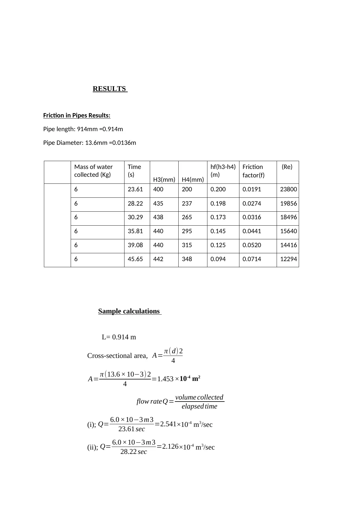
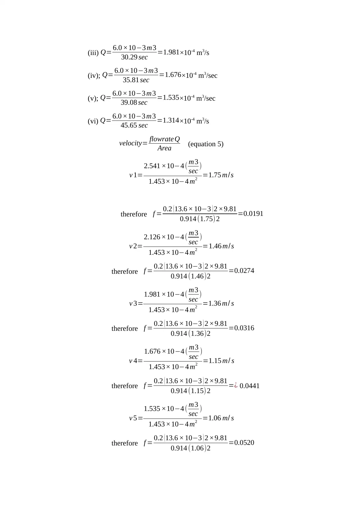
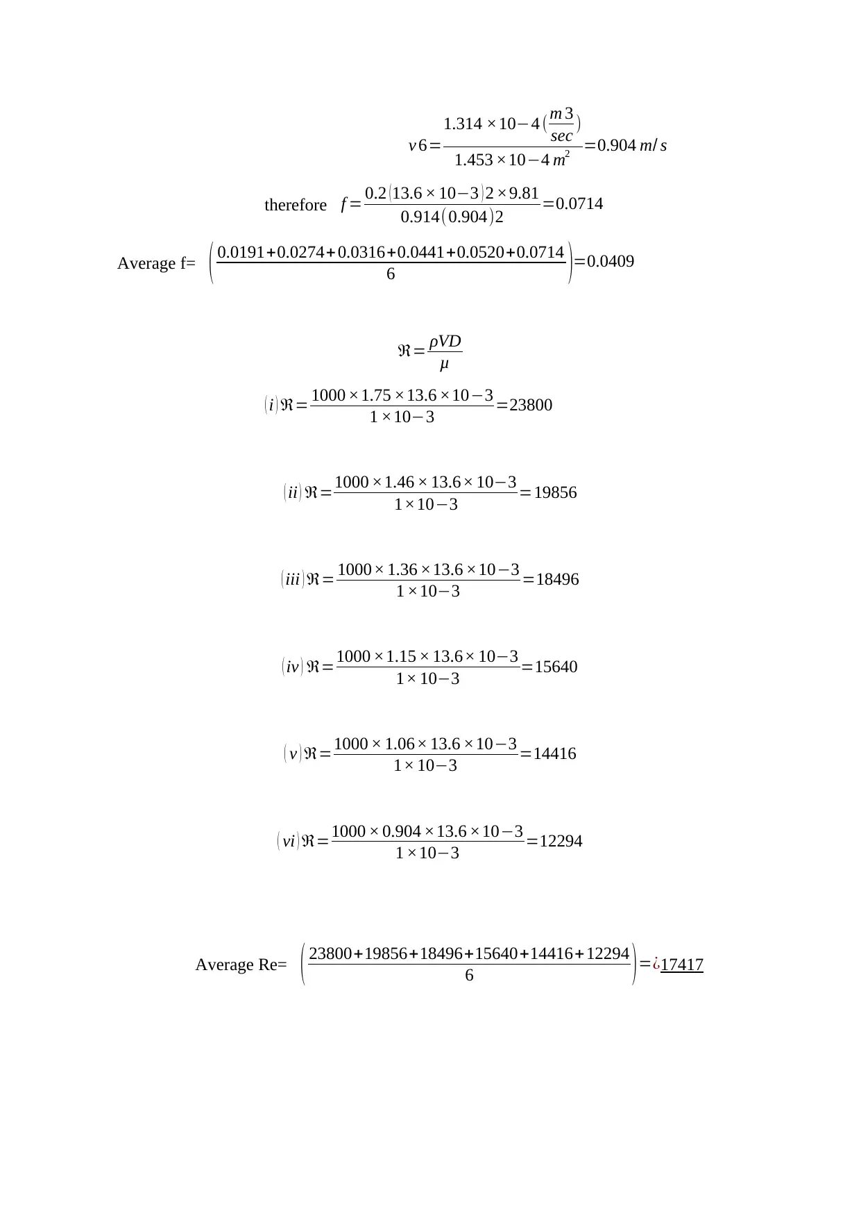
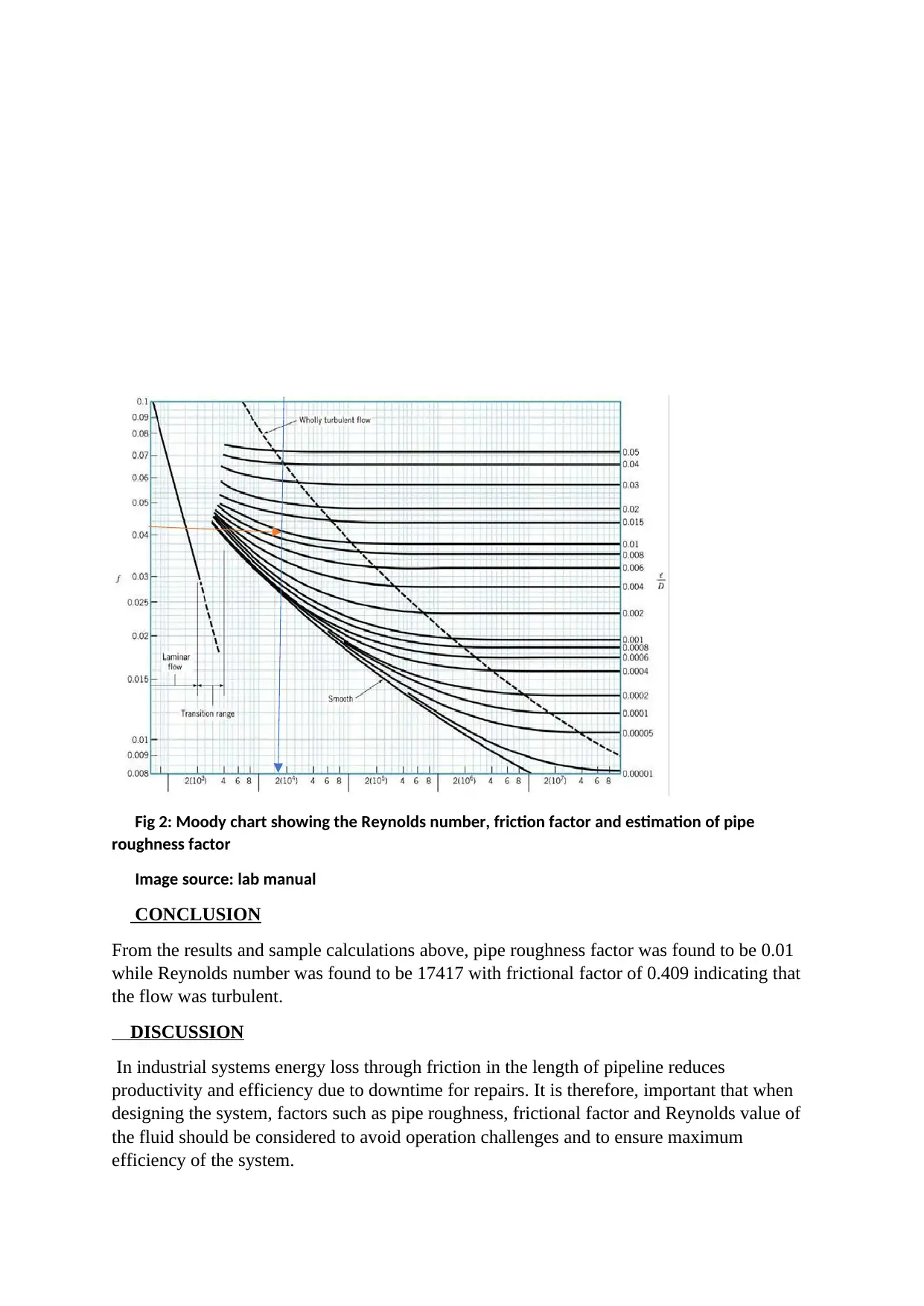
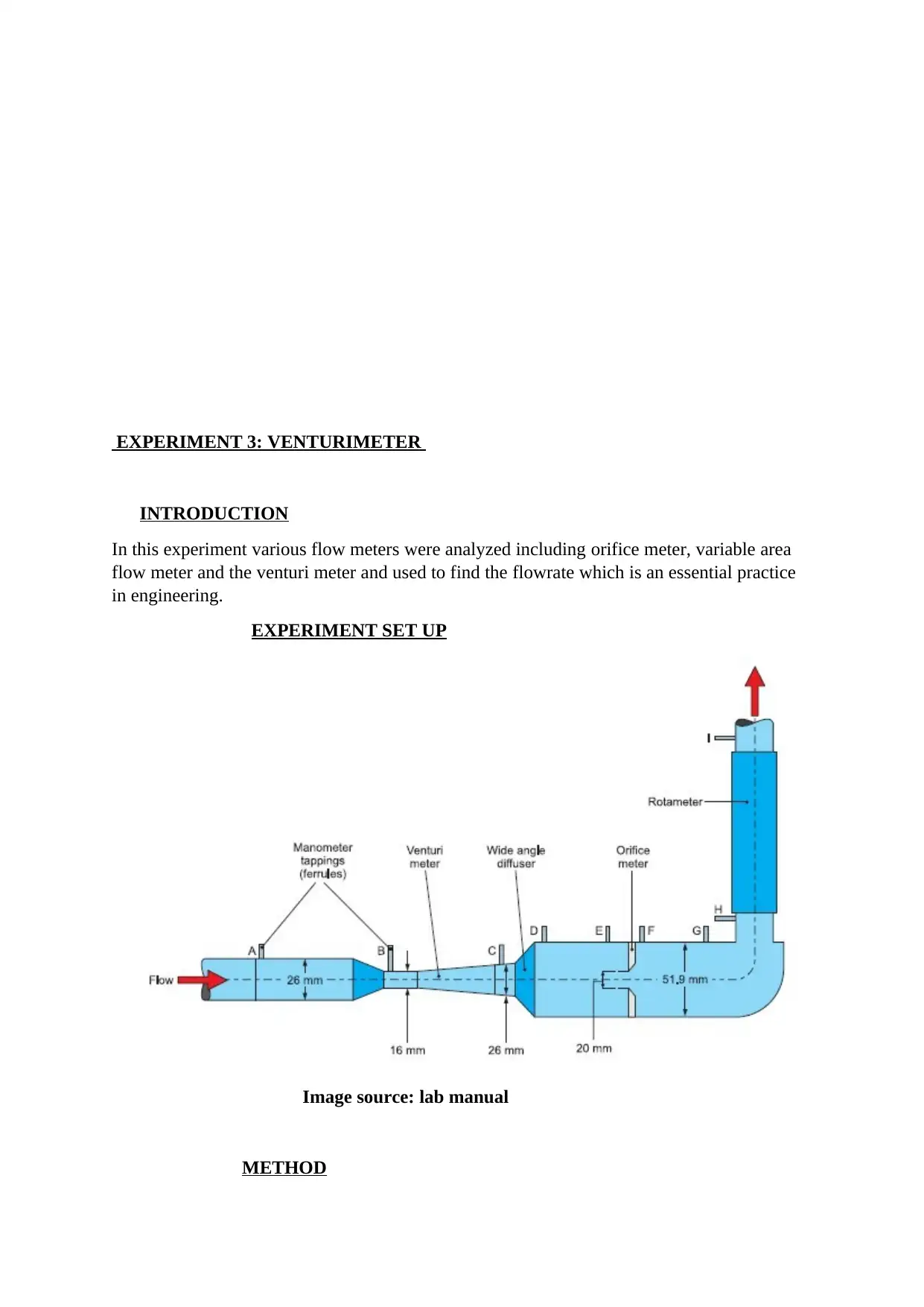
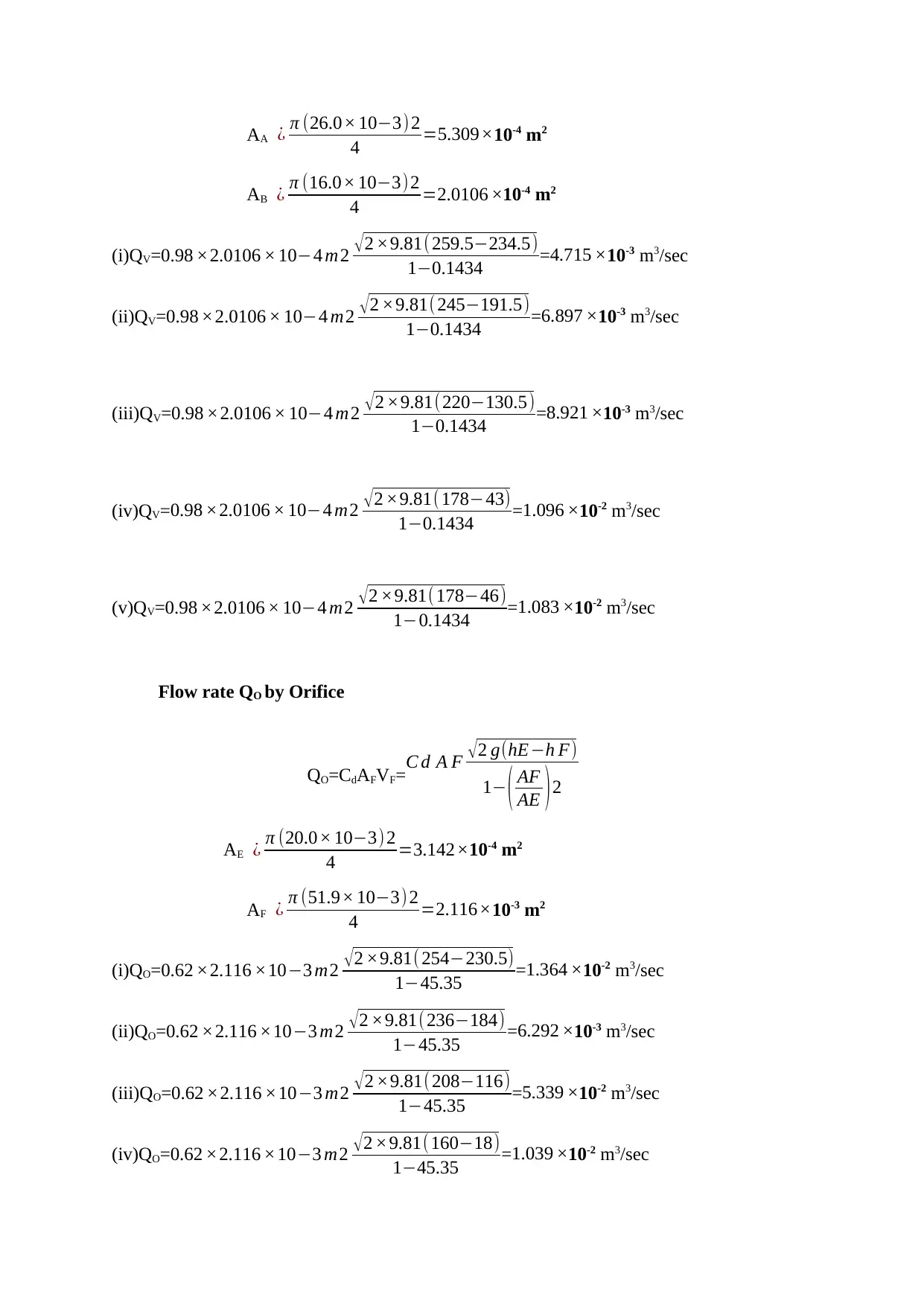
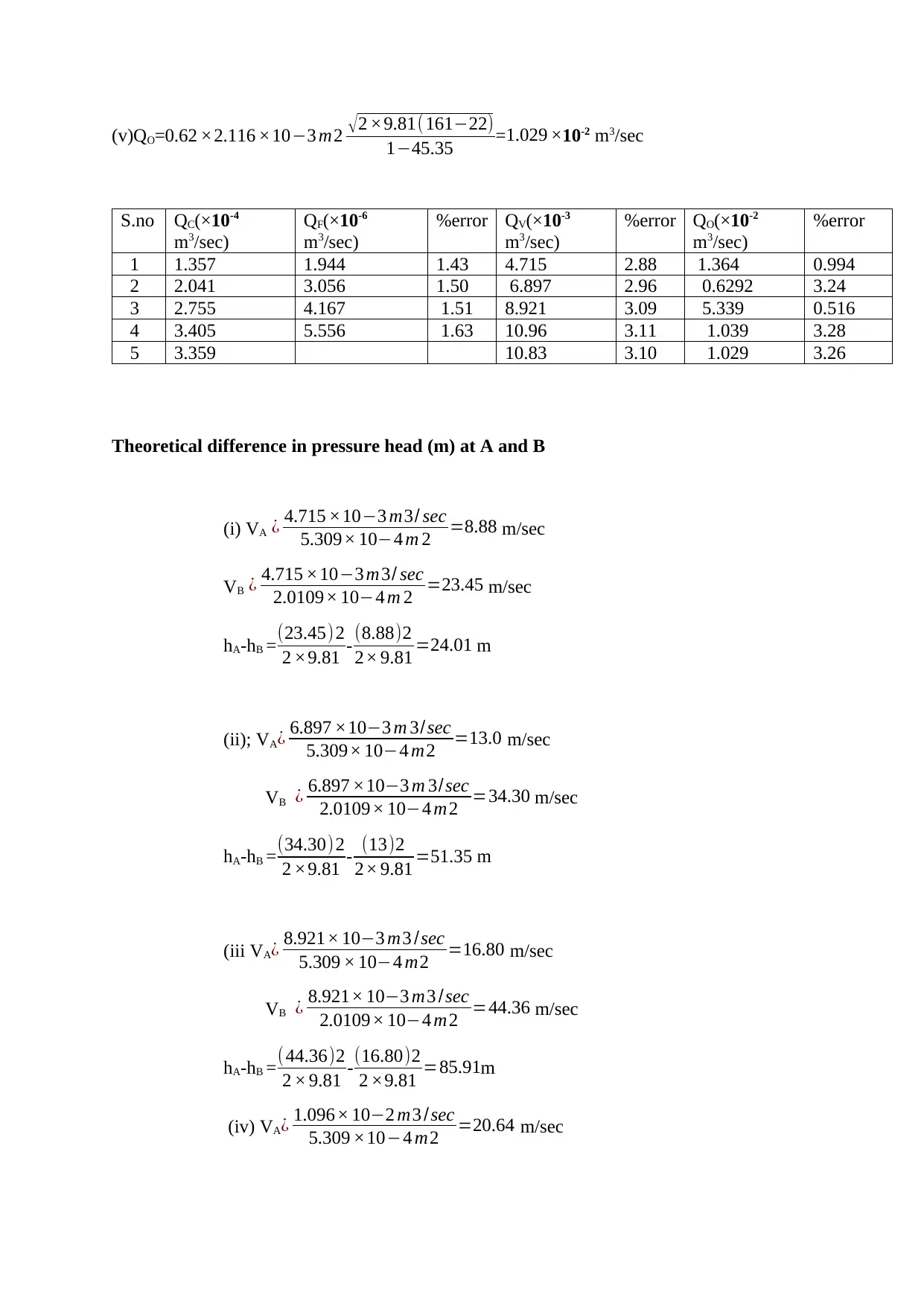
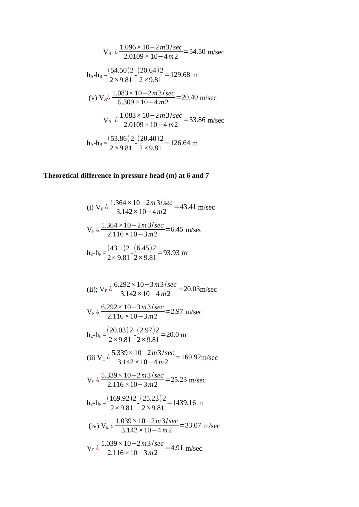
This mechanical science lab report details three experiments conducted as part of a 102MAE module at Coventry University. The first experiment investigates frictional losses in pipes, analyzing the relationship between flow rate, friction factor, and Reynolds number. The second experiment focuses on pin-jointed frames, examining stress and strain under varying loads, and calculating safety factors. The third experiment explores flow measurement using a Venturi meter and orifice plate, comparing experimental flow rates with theoretical calculations. The report includes experimental setups, methodologies, results, sample calculations, discussions, and conclusions for each experiment, providing a comprehensive analysis of the principles of fluid mechanics and structural analysis. The report also highlights potential sources of error and the practical applications of the concepts studied.

EXPERIMENT 2: FRICTION IN PIPES
INTRODUCTION
In engineering practice, it is frequently necessary to estimate the head loss incurred by a fluid
as it flows along a pipeline. In this experiment scientific knowledge gained in classwork was
applied to investigate Frictional losses experienced by a fluid as it flows through a pipe.
Experiment set up
Figure 1: pipe friction apparatus
Image source: lab manual
METHOD
Pipe friction apparatus was set up as shown above and flowrate set using the dark blue gate
valve(D)
Readings were then taken using the Gravimetric Bench and Heights of piezometers 3 and 4
recorded as shown below.

RESULTS
Friction in Pipes Results:
Pipe length: 914mm =0.914m
Pipe Diameter: 13.6mm =0.0136m
Mass of water
collected (Kg)
Time
(s) H3(mm) H4(mm)
hf(h3-h4)
(m)
Friction
factor(f)
(Re)
6 23.61 400 200 0.200 0.0191 23800
6 28.22 435 237 0.198 0.0274 19856
6 30.29 438 265 0.173 0.0316 18496
6 35.81 440 295 0.145 0.0441 15640
6 39.08 440 315 0.125 0.0520 14416
6 45.65 442 348 0.094 0.0714 12294
Sample calculations
L= 0.914 m
Cross-sectional area, A= π ( d) 2
4
A= π (13.6 × 10−3) 2
4 =1.453 ×10-4 m2
flow rateQ= volume collected
elapsed time
(i); Q= 6.0 ×10−3 m3
23.61 sec =2.541×10-4 m3/sec
(ii); Q= 6.0 ×10−3 m3
28.22 sec =2.126×10-4 m3/sec

(iii) Q= 6.0 ×10−3 m3
30.29 sec =1.981×10-4 m3/s
(iv); Q= 6.0 ×10−3 m3
35.81 sec =1.676×10-4 m3/sec
(v); Q= 6.0 ×10−3 m3
39.08 sec =1.535×10-4 m3/sec
(vi) Q= 6.0 ×10−3 m3
45.65 sec =1.314×10-4 m3/s
velocity= flowrate Q
Area (equation 5)
v 1=
2.541 ×10−4 ( m3
sec )
1.453× 10−4 m2 =1.75 m/s
therefore f = 0.2 ( 13.6 × 10−3 ) 2 ×9.81
0.914 (1.75)2 =0.0191
v 2=
2.126 ×10−4 ( m3
sec )
1.453 ×10−4 m2 =1.46 m/s
therefore f = 0.2 ( 13.6 × 10−3 ) 2 ×9.81
0.914 (1.46)2 =0.0274
v 3=
1.981 ×10−4 ( m3
sec )
1.453× 10−4 m2 =1.36 m/ s
therefore f = 0.2 ( 13.6 × 10−3 ) 2 ×9.81
0.914 (1.36)2 =0.0316
v 4=
1.676 ×10−4 ( m3
sec )
1.453× 10−4 m2 =1.15 m/ s
therefore f = 0.2 ( 13.6 × 10−3 ) 2 ×9.81
0.914 (1.15) 2 =¿ 0.0441
v 5=
1.535 ×10−4 ( m3
sec )
1.453 ×10−4 m2 =1.06 m/ s
therefore f = 0.2 ( 13.6 × 10−3 ) 2 ×9.81
0.914 (1.06)2 =0.0520

v 6=
1.314 ×10−4 (m 3
sec )
1.453 ×10−4 m2 =0.904 m/ s
therefore f = 0.2 (13.6 × 10−3 ) 2 ×9.81
0.914(0.904)2 =0.0714
Average f= ( 0.0191+0.0274+ 0.0316+0.0441+0.0520+0.0714
6 )=0.0409
ℜ= ρVD
μ
( i ) ℜ= 1000 ×1.75 ×13.6 ×10−3
1 ×10−3 =23800
( ii ) ℜ=1000 ×1.46 × 13.6× 10−3
1×10−3 =19856
( iii ) ℜ= 1000× 1.36 ×13.6 ×10−3
1 ×10−3 =18496
( iv ) ℜ=1000 ×1.15 × 13.6× 10−3
1× 10−3 =15640
( v ) ℜ=1000 × 1.06× 13.6 ×10−3
1× 10−3 =14416
( vi ) ℜ=1000 × 0.904 ×13.6 ×10−3
1 ×10−3 =12294
Average Re= ( 23800+19856+18496+15640+14416+12294
6 ) =¿17417

Fig 2: Moody chart showing the Reynolds number, friction factor and estimation of pipe
roughness factor
Image source: lab manual
CONCLUSION
From the results and sample calculations above, pipe roughness factor was found to be 0.01
while Reynolds number was found to be 17417 with frictional factor of 0.409 indicating that
the flow was turbulent.
DISCUSSION
In industrial systems energy loss through friction in the length of pipeline reduces
productivity and efficiency due to downtime for repairs. It is therefore, important that when
designing the system, factors such as pipe roughness, frictional factor and Reynolds value of
the fluid should be considered to avoid operation challenges and to ensure maximum
efficiency of the system.

EXPERIMENT 3: VENTURIMETER
INTRODUCTION
In this experiment various flow meters were analyzed including orifice meter, variable area
flow meter and the venturi meter and used to find the flowrate which is an essential practice
in engineering.
EXPERIMENT SET UP
Image source: lab manual
METHOD

The apparatus was set up as shown above and all the connections made. The values were
then collected by adjusting the flow meter valves to show readings of 50,80, 110 and 140
mm and readings of water levels in tubes A, B, C (Venturi meter), E, F (Orifice plate)
recorded.
Venturi Meter Results
SAMPLE CALCULATIONS
Analysis A: Measurement of Flow Rate

Fig: Graph 1 Rotameter Calibration Curve
Image source: lab manual
FLOAT METER (MM) FLOAT METER(L/min)
50 7
80 11
110 15
140 20
FLOAT METER (L/min) FLOW RATE QF (×10-6m3/s)
7 1.1944
11 3.056
15 4.167
20 5.556
1 L/min= 1.0× 10−3 m 3
3600 sec
(i) Qf = 7.0× 10−3 m 3
3600 sec =1.944×10-6 m3/sec
(ii) Qf = 11×10−3 m3
3600 sec =3.056×10-6 m3/sec

iii) Qf = 15× 10−3 m 3
3600 sec =4.167×10-6 m3/sec
iv) Qf = 20× 10−3 m 3
3600 sec =5.556×10-6 m3/sec
Determining QC = vol/time
VOLUME (×10-3 m3) TIME (sec) Qc (×10-4 m3/s)
6 44.2 1.357
6 29.4 2.041
6 21.78 2.755
6 17.62 3.405
12 35.72 3.359
QC = vol/time
(i) Q C=6.0 ×10−3 m3
44.2 sec =1.357×10-4 m3/sec
(ii) Q C=6.0 ×10−3 m3
29.4 sec =2.041×10-4 m3/sec
(iii) Q C=6.0 ×10−3 m3
21.78 sec =2.755×10-4 m3/sec
(iv) Q C=6.0 ×10−3 m3
17.62 sec =3.405×10-4 m3/sec
(v) Q C=6.0 ×10−3 m3
35.72 sec =3.359×10-4 m3/sec
Flow rate QV by venturi
QV=CdABVB=C d A B √2 g(hA−h B)
1−( AB
AA )2
A= π ( d) 2
4

AA ¿ π (26.0× 10−3) 2
4 =5.309×10-4 m2
AB ¿ π (16.0× 10−3)2
4 =2.0106 ×10-4 m2
(i)QV=0.98 ×2.0106 × 10−4 m2 √ 2 ×9.81( 259.5−234.5)
1−0.1434 =4.715 ×10-3 m3/sec
(ii)QV=0.98 ×2.0106 × 10−4 m2 √ 2 ×9.81(245−191.5)
1−0.1434 =6.897 ×10-3 m3/sec
(iii)QV=0.98 ×2.0106 × 10−4 m2 √ 2 ×9.81(220−130.5)
1−0.1434 =8.921 ×10-3 m3/sec
(iv)QV=0.98 ×2.0106 × 10−4 m2 √2 ×9.81( 178−43)
1−0.1434 =1.096 ×10-2 m3/sec
(v)QV=0.98 ×2.0106 × 10−4 m2 √ 2 ×9.81(178−46)
1−0.1434 =1.083 ×10-2 m3/sec
Flow rate QO by Orifice
QO=CdAFVF=
C d A F √ 2 g(hE−h F)
1− ( AF
AE ) 2
AE ¿ π (20.0× 10−3) 2
4 =3.142×10-4 m2
AF ¿ π (51.9× 10−3) 2
4 =2.116×10-3 m2
(i)QO=0.62 ×2.116 ×10−3 m2 √2 ×9.81( 254−230.5)
1−45.35 =1.364 ×10-2 m3/sec
(ii)QO=0.62 ×2.116 ×10−3 m2 √2 ×9.81( 236−184)
1−45.35 =6.292 ×10-3 m3/sec
(iii)QO=0.62 ×2.116 ×10−3 m2 √ 2 ×9.81( 208−116)
1−45.35 =5.339 ×10-2 m3/sec
(iv)QO=0.62 ×2.116 ×10−3 m2 √2 ×9.81(160−18)
1−45.35 =1.039 ×10-2 m3/sec

(v)QO=0.62 ×2.116 ×10−3 m2 √2 ×9.81( 161−22)
1−45.35 =1.029 ×10-2 m3/sec
S.no QC(×10-4
m3/sec)
QF(×10-6
m3/sec)
%error QV(×10-3
m3/sec)
%error QO(×10-2
m3/sec)
%error
1 1.357 1.944 1.43 4.715 2.88 1.364 0.994
2 2.041 3.056 1.50 6.897 2.96 0.6292 3.24
3 2.755 4.167 1.51 8.921 3.09 5.339 0.516
4 3.405 5.556 1.63 10.96 3.11 1.039 3.28
5 3.359 10.83 3.10 1.029 3.26
Theoretical difference in pressure head (m) at A and B
(i) VA ¿ 4.715 ×10−3 m3/ sec
5.309× 10−4 m 2 =8.88 m/sec
VB ¿ 4.715 ×10−3 m3/ sec
2.0109× 10−4 m 2 =23.45 m/sec
hA-hB = (23.45)2
2 ×9.81 - (8.88)2
2× 9.81 =24.01 m
(ii); VA¿ 6.897 ×10−3 m 3/sec
5.309× 10−4 m2 =13.0 m/sec
VB ¿ 6.897 ×10−3 m 3/sec
2.0109× 10−4 m2 =34.30 m/sec
hA-hB = (34.30)2
2 ×9.81 - (13)2
2× 9.81 =51.35 m
(iii VA¿ 8.921× 10−3 m3 /sec
5.309 × 10−4 m2 =16.80 m/sec
VB ¿ 8.921× 10−3 m3 /sec
2.0109× 10−4 m2 =44.36 m/sec
hA-hB =(44.36)2
2 × 9.81 -(16.80)2
2 ×9.81 =85.91m
(iv) VA¿ 1.096× 10−2 m3 /sec
5.309 ×10−4 m2 =20.64 m/sec

VB ¿ 1.096× 10−2 m3 /sec
2.0109 × 10−4 m2 =54.50 m/sec
hA-hB =(54.50)2
2 ×9.81 -(20.64)2
2 ×9.81 =129.68 m
(v) VA¿ 1.083× 10−2 m3 / sec
5.309 ×10−4 m2 =20.40 m/sec
VB ¿ 1.083× 10−2 m3 /sec
2.0109 ×10−4 m2 =53.86 m/sec
hA-hB =(53.86) 2
2 ×9.81 -(20.40)2
2 ×9.81 =126.64 m
Theoretical difference in pressure head (m) at 6 and 7
(i) VE ¿ 1.364 ×10−2m 3/sec
3.142× 10−4 m2 =43.41 m/sec
VF ¿ 1.364 ×10−2m 3/ sec
2.116 ×10−3 m2 =6.45 m/sec
hE-hF = (43.1)2
2× 9.81- (6.45)2
2× 9.81 =93.93 m
(ii); VE ¿ 6.292× 10−3 m3 /sec
3.142×10−4 m2 =20.03m/sec
VF ¿ 6.292× 10−3 m3 / sec
2.116 ×10−3 m2 =2.97 m/sec
hE-hF =(20.03)2
2 ×9.81 - (2.97)2
2× 9.81 =20.0 m
(iii VE ¿ 5.339× 10−2 m3 /sec
3.142 ×10−4 m2 =169.92m/sec
VF ¿ 5.339× 10−2 m3 / sec
2.116 ×10−3 m2 =25.23 m/sec
hE-hF =(169.92)2
2× 9.81 - (25.23) 2
2 ×9.81 =1439.16 m
(iv) VE ¿ 1.039× 10−2 m3 /sec
3.142 ×10−4 m2 =33.07 m/sec
VF ¿ 1.039× 10−2 m3 /sec
2.116 ×10−3 m2 =4.91 m/sec

hE-hF =(33.07)2
2 ×9.81 - (4.91)2
2× 9.81 =54.51m
(v) VE ¿ 1.029× 10−2 m3 /sec
3.142 ×10−4 m2 =32.75m/sec
VF ¿ 1.029× 10−2 m3 / sec
2.116 ×10−3 m2 =4.86 m/sec
hE-hF = (32.75)2
2 ×9.81 - ( 4.86)2
2× 9.81 =53.47 m
S.no Theoretical
pressure head
(Venturi)
(m)
Experiment
pressure
head (hA-hB)
(m)
%
error
S.no Theoretical
pressure
head
(Orifice)
(m)
Experiment
pressure
head (hE-hF)
(m)
%
error
1 24.01 25 4.13 1 93.93 23.5 74.98
2 51.35 53.5 4.19 2 20 52 160
3 85.91 89.5 4.18 3 1439.16 92 93.61
4 129.68 135 4.10 4 54.2 142 162
5 126.64 132 4.23 5 53.47 139 160
DISCUSSION
A huge error in differential pressure head of orifice meter is noticed on comparing it with
theoretical calculations. This may have accoutred due to experimental errors
On comparing the theoretical results of venturi-meter and experimental values, a slight
difference is noted and an error ranging from 4.10% and 4.23%
CONCLUSION
The experiment was carried out successfully and it enable one to apply the scientific
knowledge learned in classroom to solve real world problems and also to analyse the system
and find out its efficiency in terms of errors.

EXPERIMENT 1: PIN-JOINTED FRAMES
INTRODUCTION
Trusses and frames are used as simple skeletal structures and act as pin-joined frame.
Individual members of truss are subject to tensional and compressional forces without
bending moments. In this experiment we apply scientific knowledge learned to analyse
frames and find safety factor.
Fig 1: The Warren Girder structure
Image source: lab manual
Experiment set up
Fig 2: pin jointed frames
Image source: https://www.tecquipment.com/pin-jointed-frameworks

METHOD
The equipment was set up as shown and preload of 100 N and the load cell set to zero
A load of 500 N was Carefully applied and frame checked for stability and loads applied in
increments of 100 N, then strain readings for each member tabulated in Table 1a.
RESULTS
Load (N) Strain
Gauge 1
Strain
Gauge 2
Strain
Gauge 3
Strain
Gauge 4
Strain
Gauge 5
0 0 -3 -1 0 1
100 -21 -14 -6 13 12
200 -42 -28 -11 26 23
300 -64 -40 -15 39 35
400 -86 -51 -21 52 47
500 -109 -63 -27 64 60
TABLE 1a
SAMPLE CALCULATIONS
Analysis of pin jointed frame
JOINT D

∑ FY =0
FDCSIN60-500=0
FDC= 500
sin 60=577.35N
∑ FX=0
FDB-577.35COS60=0
FDB=288.68N
JOINT B
∑ FY =0
FBCSIN60- FBASIN60=0
FBC=FBA=F=577.35N
∑ FX=0
577.35-2FCOS60=0
F=577.35N
JOINT C
∑ FY =0
Cy-2(577.35SIN60) =0
CY=1000N
∑ FX=0
FCA+577.35COS60-577.35COS60-288.68=0
FCA=288.68N
JOINT A
∑ FY =0
FABSIN60- FA=0

FA=577.35SIN60
FA=500N
1 2 3 4 5
Theoretical Force, N 577.35 577.35 288.68 288.68 577.35
Experimental Force, N 647.78 374.41 160 380 356.58
Experimental stress, (MN/M2) 22.89 13.23 5.65 13.43 12.61
experimental force,
F = A E ε
(I) F = 28.3 x 10−6 ×210 ×10 9 ×109 x 10−6 = 647.78N (C)
(ii) F = 28.3 x 10−6 ×210 ×10 9 ×63 x 10−6 = 374.41N (C)
(iii) F = 28.3 x 10−6 ×210 ×10 9 ×27 x 10−6 = 160N (C)
(iv) F = 28.3 x 10−6 ×2 10× 10 9 ×64 x 10−6 = 380N (T)
(v) F = 28.3 x 10−6 ×210 ×10 9 ×60 x 10−6 = 356.58N (T)
experimental stress: σ = F
A (N/M2)
( i ) σ= 647.78
28.3 ×10−6 =22.89 ×10 6 N / M 2
(ii) σ = 374.41
28.3× 10−6 =13.23× 10 6 N /M 2
(ii) σ = 160
28.3× 10−6 =5.65× 10 6 N /M 2
(iv) σ = 380
28.3× 10−6 =13.43× 10 6 N /M 2

(v) σ = 356.58
28.3× 10−6 =12.61×10 6 N /M 2
Factor of safety of 500N
S.F= YIELD STRESS
ACTUAL STRESS
(i) S.F = 400 ×106
22.89× 106 =¿17.5
(ii) S.F = 400 ×106
13.23× 106 =¿30.2
(iii) S.F = 400 ×106
5.65× 106 =¿70.8
(Iv) S.F = 400 ×106
13.43× 106 =¿29.8
(v) S.F = 400× 106
12.61×106 =¿31.7
1 2 3 4 5
Strain(με) -109 -60 -26 64 59
Table 1b Increase in Strain, 500 N –0 N loading (με)

GRAPH
0 100 200 300 400 500 600
0
10
20
30
40
50
60
70
STRAIN AGAINST LOAD
strain1
strain2
strain3
strain4
strain5
LOAD(N)
STRSIN
DISCUSSION
From data analysis a graph of load against strain gives a straight line passing through the
origin it shows that frames 1,2 & 3 are subjected to compression while 4 & 5 are subjected to
tension.
Comparing the experiment results to that of theoretical analysis a slight difference is seen,
this may have resulted due to the experimental errors.
From stress analysis the scientific-theory is confirmed that stress increase with increase in
load for a constant cross-sectional.
The level of safety for a load of 500N on each member is very high when Yield Stress of 400
MN/m2 is used therefore, ensuring user safety and longer lasting to the equipment.
CONCLUSION
After carrying out the experiment and data analysis of truss frames it is concluded that
analysis of every frame in construction design, is crucial and should be carried out effectively
to find out the stress that each frame is subjected to and there after recommend a safety factor
to avoid accidents due to collapse of the structures.
REFERENCES
B. R. Munson, D.F Young and T. H. Okiis shi,( 2010) Fundamentals of Fluid Mechanics.
John Wiley and Sons, Inc.
F.M White. (2013 October). Fluid Mechanics 3nd Edition. McGraw-Hill

S. Ramachandran and V.Saikrishnan. (2014). fluid mechanics and machinery (2nd Edition).
Wellington New Zealand.
Hill, A., & Ladson, C.M, (2013). Pressure distribution from high Reynold numbers. NASA
TM 100526
Mabie, H. H., Mechanisms and Dynamics of Machines
Prentice, J. M., Dynamics of Mechanical Systems.
Hamilton, H.M and Charles F.R., Mechanics and Dynamics of Machinery,
Shigley J. and Uicker, Theory of Machines and Mechanisms,